3
play

3 Short review Lecture no: NARROW-BAND CHANNELS WIDE-BAND - PowerPoint PPT Presentation

RADIO SYSTEMS ETI 051 Contents 3 Short review Lecture no: NARROW-BAND CHANNELS WIDE-BAND CHANNELS Radio signals and complex Delay (time) dispersion notation Narrow- versus wide-band Large-scale fading channels


  1. RADIO SYSTEMS – ETI 051 Contents 3 • Short review Lecture no: NARROW-BAND CHANNELS WIDE-BAND CHANNELS • Radio signals and complex • Delay (time) dispersion notation • Narrow- versus wide-band • Large-scale fading channels Narrow- and wideband • Small-scale fading • The WSSUS model • Combining large- and small- – Wide-sense stationary (US) channels scale fading – Uncorrelated scatterers (US) – Tapped delay line models • Noise- and interference- limited links • Condensed parameters – Some system functions – Window parameters Ove Edfors, Department of Electrical and Information technology Ove.Edfors@eit.lth.se 2010-03-23 Ove Edfors - ETI 051 1 2010-03-23 Ove Edfors - ETI 051 2 
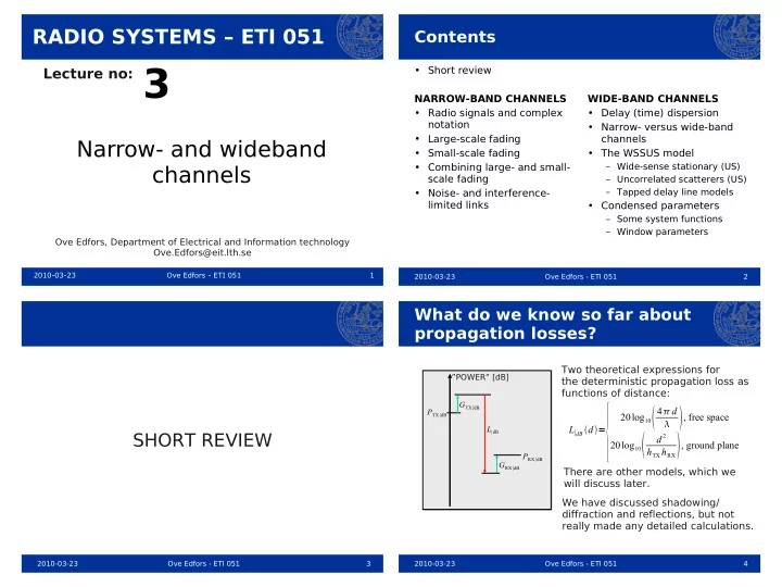
What do we know so far about propagation losses? Two theoretical expressions for ”POWER” [dB] the deterministic propagation loss as functions of distance: L ∣ dB  d = { G TX ∣ dB 20log 10    , free space 4  d P TX ∣ dB L ∣ dB 20log 10  h TX h RX  , ground plane SHORT REVIEW 2 d P RX ∣ dB G RX ∣ dB There are other models, which we will discuss later. We have discussed shadowing/ diffraction and reflections, but not really made any detailed calculations. 2010-03-23 Ove Edfors - ETI 051 3 2010-03-23 Ove Edfors - ETI 051 4

  2. Statistical descriptions of the mobile radio channel The propagation ”POWER” [dB] loss will change due to movements. G TX ∣ dB P TX ∣ dB L ∣ dB These changes of the propagation RADIO SIGNALS AND loss will take place in two scales: COMPLEX NOTATION P RX ∣ dB Large-scale: shadowing, “slow” G RX ∣ dB changes over many wavelengths . Small-scale: interference, “fast” changes on the scale of a wavelength. Now we are going to approach these variations from a statistical point of view. 2010-03-23 Ove Edfors - ETI 051 5 2010-03-23 Ove Edfors - ETI 051 6 Simple model of a radio signal The IQ modulator ( ) • A transmitted radio signal can be written s t I I-channel ( ) ( ) ( ) Transmited radio signal (in-phase) π cos 2 f t = π + φ s t A cos 2 ft c ( ) ( ) ( ) f = π s t s t cos 2 f t c I c ( ) ( ) − π s t sin 2 f t Amplitude Frequency Phase Q c o • By letting the transmitted information change the -90 ( ) ( ) − π sin 2 f t amplitude, the frequency, or the phase, we get the s t c Q Q-channel tree basic types of digital modulation techniques (quadrature) Take a step into the complex domain: – ASK (Amplitude Shift Keying) s  t = s I  t  j s Q  t   Complex envelope – FSK (Frequency Shift Keying) s  t = Re {  j 2  f c t } s  t  e Constant amplitude – PSK (Phase Shift Keying) j 2 π f t Carrier factor e c 2010-03-23 Ove Edfors - ETI 051 7 2010-03-23 Ove Edfors - ETI 051 8

  3. Interpreting the complex Example: Amplitude, phase and notation frequency modulation ( ) ( ) ( ) ( ) = π + φ s t A t cos 2 f t t Complex envelope (phasor) Transmitted radio signal c ( ) ( ) φ Q A t t Comment: ( ) s t  s  t  00 01 11 00 10 Re {  j 2  f c t } Q s  t  = s  t  e ( ) - Amplitude carries information ( ) A t φ t 4ASK Re { A  t  e j 2  f c t } - Phase constant (arbitrary) j  t  e = ( ) I s t Re { A  t  e j  2  f c t  t  } = I 00 01 11 00 10 = A  t  cos  2  f c t  t  - Amplitude constant (arbitrary) 4PSK - Phase carries information Polar coordinates: By manipulating the amplitude A (t) j  t  00 01 11 00 10 s  t = s I  t  j s Q  t = A  t  e  and the phase Φ (t) of the complex - Amplitude constant (arbitrary) envelope (phasor), we can create any - Phase slope (frequency) type of modulation/radio signal. 4FSK carries information 2010-03-23 Ove Edfors - ETI 051 9 2010-03-23 Ove Edfors - ETI 051 10 A narrowband system described in complex notation (noise free) Transmitter Channel Receiver ( ) ( ) x t y t ( ) ( ) ( ) ( ) ( ) α θ π t exp j t − π exp j 2 f exp j 2 f LARGE-SCALE c c FADING Attenuation Phase ( ) ( ) ( ) ( ) = φ In: x t A t exp j t ( ) ( ) ( ) ( ) ( ) ( ) ( ) ( ) ( ) Out: = φ π α θ − π y t A t exp j t exp j 2 f t t exp j t exp j 2 f t c c ( ) ( ) ( ) ( ) ( ) ( ) = α φ + θ A t t exp j t t It is the behaviour of the channel attenuation and phase we are going to model. 2010-03-23 Ove Edfors - ETI 051 11 2010-03-23 Ove Edfors - ETI 051 12

  4. Large-scale fading Large-scale fading Basic principle More than one shadowing object Signal path in terrain with several diffraction points adding extra attenuation to the pathloss. This is ONE Received power explanation α N D α α C 1 2 d B Movement Total pathloss: L tot = L  d × 1 × 2 ×⋯× N A If these are considered Position random and independent, A B C C we should get a normal L tot ∣ dB = L  d  ∣ dB  1 ∣ dB  2 ∣ dB ⋯ N ∣ dB distribution in the dB domain. Deterministic 2010-03-23 Ove Edfors - ETI 051 13 2010-03-23 Ove Edfors - ETI 051 14 Large-scale fading Large-scale fading Log-normal distribution Fading margin Measurements confirm that in many situations, the large-scale We know that the path loss will vary around the deterministic value fading of the received signal strength has a normal distribution predicted. in the dB domain. ( ) Note dB pdf L | dB scale ”POWER” [dB] We need to design our system with a “margin” allowing us to handle higher path losses than the deterministic prediction. This margin is called a fading margin . P TX ∣ dB L ∣ dB dB Deterministic mean value of path loss, L 0 Increasing the fading margin decreases the probability of outage , |d B which is the probability that our system receive a too low power P RX ∣ dB exp  −  L ∣ dB − L 0 ∣ dB   2 to operate correctly. 1 pdf  L ∣ dB  =  2  F ∣ dB 2 2  F ∣ dB Standard deviation  F ∣ dB ≈ 4 − 10 dB 2010-03-23 Ove Edfors - ETI 051 15 2010-03-23 Ove Edfors - ETI 051 16

  5. Large-scale fading The Q(.)-function Fading margin (cont.) Upper-tail probabilities Fading margin x Q(x) x Q(x) x Q(x) M Designing the system to handle | dB 4.265 0.00001 3.090 0.00100 1.282 0.10000 an M |d B higher loss than ( ) pdf L 4.107 0.00002 2.878 0.00200 0.842 0.20000 predicted, | dB 4.013 0.00003 2.748 0.00300 0.524 0.30000 lowers the probability of outage. 3.944 0.00004 2.652 0.00400 0.253 0.40000 P out = Pr { L ∣ dB  L 0 ∣ dB  M ∣ dB } = Q   F ∣ dB  M ∣ dB 3.891 0.00005 2.576 0.00500 0.000 0.50000 3.846 0.00006 2.512 0.00600 3.808 0.00007 2.457 0.00700 3.775 0.00008 2.409 0.00800 dB L 3.746 0.00009 2.366 0.00900 0| dB 3.719 0.00010 2.326 0.01000 The upper tail probability of a unit variance, 3.540 0.00020 2.054 0.02000 zero-mean, Gaussian (normal) variable: 3.432 0.00030 1.881 0.03000 3.353 0.00040 1.751 0.04000  2  exp  − x 2  dx = 1 2 erfc   2  ∞ 2 1 y 3.291 0.00050 1.645 0.05000 Q  y = ∫ 3.239 0.00060 1.555 0.06000 y 3.195 0.00070 1.476 0.07000 3.156 0.00080 1.405 0.08000 The complementary error-function 3.121 0.00090 1.341 0.09000 can be found in e.g. MATLAB 2010-03-23 Ove Edfors - ETI 051 17 2010-03-23 Ove Edfors - ETI 051 18 Large-scale fading A numeric example How many dB fading margin, against σ F = 7 dB log-normal fading, do |d B we need to obtain an outage probability of 0.5%? P out = Q   F ∣ dB  M ∣ dB = = 0.5% 0.005 SMALL-SCALE FADING Consulting the Q(.)-function table (or using a numeric software), we get M ∣ dB = 2.576 ⇒ M ∣ dB = 2.576 ⇒ M ∣ dB = 18  F ∣ dB 7 2010-03-23 Ove Edfors - ETI 051 19 2010-03-23 Ove Edfors - ETI 051 20

  6. Small-scale fading Small-scale fading Two waves Ilustration shown during Lecture 1 Illustration of interference pattern from above Received power [log scale] Wave 1 Movement A B Wave 1 + Wave 2 Position Transmitter Wave 2 A B Reflector λ At least in this case, we can see that the interference pattern changes on the wavelength scale. Many reflectors ... let’s look at a simpler case! 2010-03-23 Ove Edfors - ETI 051 21 2010-03-23 Ove Edfors - ETI 051 22 Small-scale fading Small-scale fading Many incoming waves Rayleigh fading Many incoming waves with Add them up as phasors No dominant component TX RX X independent amplitudes (no line-of-sight) and phases Tap distribution Amplitude distribution 2D Gaussian  3 Rayleigh (zero mean) r φ ,  2 r 2 2 r φ , 0.8 2 1 1 r  1 φ r 1 0.6 3 r ( ) ( ) Im a Re a = 0.4 r φ r a , 4 4 r φ , 0.2 3 3 r  4 r φ , 4 0 0 1 2 3 2 exp  − r 2  2 pdf  r = r ( ) ( ) ( ) ( ) ( ) φ = φ + φ + φ + φ r exp j r exp j r exp j r exp j r exp j 1 1 2 2 3 3 4 4 No line-of-sight  2  component 2010-03-23 Ove Edfors - ETI 051 23 2010-03-23 Ove Edfors - ETI 051 24

Download Presentation
Download Policy: The content available on the website is offered to you 'AS IS' for your personal information and use only. It cannot be commercialized, licensed, or distributed on other websites without prior consent from the author. To download a presentation, simply click this link. If you encounter any difficulties during the download process, it's possible that the publisher has removed the file from their server.

Recommend


More recommend