3.3 Index Access Scheduling Given: index scans over m lists L i - PowerPoint PPT Presentation

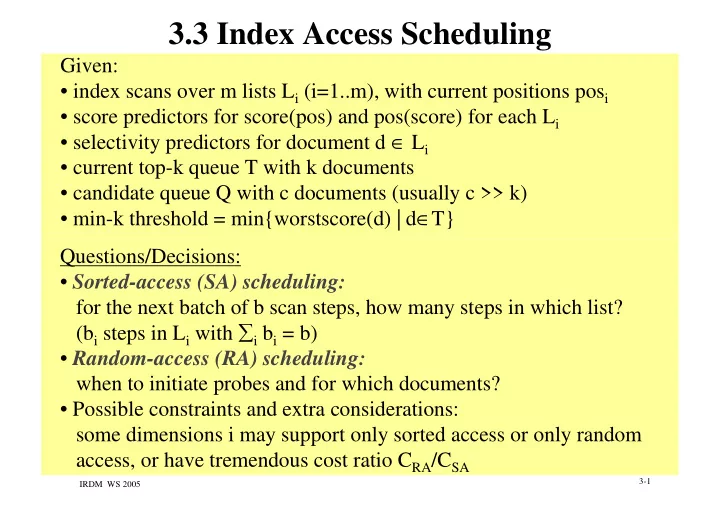
3.3 Index Access Scheduling Given: • index scans over m lists L i (i=1..m), with current positions pos i • score predictors for score(pos) and pos(score) for each L i • selectivity predictors for document d ∈ L i • current top-k queue T with k documents • candidate queue Q with c documents (usually c >> k) • min-k threshold = min{worstscore(d) | d ∈ T} Questions/Decisions: • Sorted-access (SA) scheduling: for the next batch of b scan steps, how many steps in which list? (b i steps in L i with ∑ i b i = b) • Random-access (RA) scheduling: when to initiate probes and for which documents? • Possible constraints and extra considerations: some dimensions i may support only sorted access or only random access, or have tremendous cost ratio C RA /C SA 3-1 IRDM WS 2005

Combined Algorithm (CA) assume cost ratio C RA /C SA = r perform NRA (TA-sorted) with [worstscore, bestscore] bookkeeping in priority queue Q and round-robin SA to m index lists ... after every r rounds of SA (i.e. m*r scan steps) perform RA to look up all missing scores of „best candidate“ in Q (where „best“ is in terms of bestscore, worstscore, or E[score], or P[score > min-k]) cost competitiveness w.r.t. „optimal schedule“ (scan until Σ Σ i high i ≤ min{bestscore(d) | d ∈ ∈ final top-k}, Σ Σ ∈ ∈ then perform RAs for all d‘ with bestscore(d‘) > min-k): 4m + k 3-2 IRDM WS 2005

Sorted-Access Scheduling available info: L 1 L 2 L 3 L 4 L i ... ... 0.9 0.9 0.9 0.9 100 100 100 100 0.8 0.9 0.9 0.8 score 200 pos i 200 200 200 (pos i ) 0.7 0.8 0.8 0.6 300 300 300 300 µ i µ µ µ 0.6 0.8 0.8 0.4 δ i δ δ δ 400 400 400 400 pos i 0.5 0.7 0.6 0.3 500 score 500 500 500 +b i (b i + 0.4 0.7 0.4 0.2 600 600 600 600 pos i ) 0.3 0.6 0.2 0.1 700 700 700 700 0.2 0.6 0.1 0.05 800 800 800 800 0.1 0.5 0.05 0.01 900 900 900 900 goal: eliminate candidates quickly aim for quick drop in high i bounds 3-3 IRDM WS 2005

SA Scheduling: Objective and Heuristics plan next b 1 , ..., b m index scan steps for batch of b steps overall s.t. Σ Σ i=1..m b i = b Σ Σ and benefit(b 1 , ..., b m ) is max! possible benefit definitions: = ∆ ∆ = − + with benefit ( b .. b ) ( high score ( pos b )) / b ∑ = 1 m i i i i i i i i 1 .. m score gradient = δ δ = − + benefit ( b .. b ) with score ( pos ) score ( pos b ) ∑ = 1 m i i 1 .. m i i i i i i score reduction Solve knapsack-style NP-hard optimization problem (e.g. for batched scans) or use greedy heuristics: b i := b * benefit(b i =b) / ∑ ν ν =1..m benefit(b ν ν =b) ν ν ν ν 3-4 IRDM WS 2005

SA Scheduling: Benefit Aggregation Heuristics Consider current top-k T and andidate queue Q; for each d ∈ ∈ T ∪ ∈ ∈ ∪ Q we know E(d) ⊆ ∪ ∪ ⊆ 1..m, R(d) = 1..m – E(d), ⊆ ⊆ bestscore(d), worstscore(d), p(d) = P[score(d) > min-k] = = = = ( , .. ) benefit d b b score 1 m − − − − ⋅ ⋅ − − + + ⋅ ⋅ − − + + 1 ( ) ( ( )) surplus d high score pos b current top-k candidates in ∑ ∉ ∉ ∉ ∉ i i i ( ) i E d Q − ⋅ + + + + − − − ⋅ ⋅ ⋅ µ µ µ µ 1 bestscore(d) ( ) gap d ∑ ∉ ∉ ∉ ∉ i i E ( d ) plus(d) Sur- with surplus(d) = bestscore(d) – min-k gap(d) = min-k – worstscore(d) min-k µ i = E[score(j) | j ∈ [pos i , pos i +b i ]] gap(d) = benefit ( b .. b ) benefit ( d , b .. b ) ∑ worstscore(d) 1 m ∈ ∪ 1 m d T Q weighs documents and dimensions in benefit function 3-5 IRDM WS 2005

Random-Access Scheduling: Heuristics Perform additional RAs when helpful 1) to increase min-k (increase worstscore of d ∈ ∈ top-k) or ∈ ∈ 2) to prune candidates (decrease bestscore of d ∈ ∈ ∈ Q) ∈ For 1) Top Probing: • perform RAs for current top-k (whenever min-k changes), • and possibly for best d from Q (in desc. order of bestscore, worstscore, or P[score(d)>min-k]) For 2) 2-Phase Probing: perform RAs for all candidates at point t total cost of remaining RAs = total cost of SAs up to t (motivated by linear increase of SA-cost(t) and sharply decreasing remaining-RA-cost(t)) 3-6 IRDM WS 2005

Top-k Queries over Web Sources Typical example: Address = „2590 Broadway“ and Price = $ 25 and Rating = 30 issued against mapquest.com, nytoday.com, zagat.com Major complication: some sources do not allow sorted access highly varying SA and RA costs Major opportunity: sources can be accessed in parallel → → → → extension/generalization of TA distinguish S-sources, R-sources, SR-sources 3-7 IRDM WS 2005

Source-Type-Aware TA For each R-source S i ∈ S m+1 .. S m+r set high i := 1 Scan SR- or S-sources S 1 .. S m Choose SR- or S-source S i for next sorted access for object d retrieved from SR- or S-source L i do { E(d) := E(d) ∪ {i}; high i := si(q,d); bestscore(d) := aggr{x1, ..., xm) with xi := si(q,d) for i ∈ E(d), high i for i ∉ E(d); worstscore(d) := aggr{x1, ..., xm) with xi := si(q,d) for i ∈ E(d), 0 for i ∉ E(d); }; Choose SR- or R-source Si for next random access for object d retrieved from SR- or R-source L i do { E(d) := E(d) ∪ {i}; bestscore(d) := aggr{x1, ..., xm) with xi := si(q,d) for i ∈ E(d), high i for i ∉ E(d); worstscore(d) := aggr{x1, ..., xm) with xi := si(q,d) for i ∈ E(d), 0 for i ∉ E(d); }; current top-k := k docs with largest worstscore; min-k := minimum worstscore among current top-k; Stop when bestscore(d | d not in current top-k results) ≤ min-k ; Return current top-k; essentially NRA with choice of sources 3-8 IRDM WS 2005

Strategies for Choosing the Source for Next Access for next sorted acccess: Escore(Li) := expected si value for next sorted access to Li (e.g.: high i ) rank(Li) := w i * Escore(Li) / c SA (Li) // w i is weight of Li in aggr // c SA (Li) is source-specific SA cost choose SR- or S-source with highest rank(Li) for next random acccess (probe): Escore(Li) := expected si value for next random access to Li (e.g.: (high i − low i ) / 2) rank(Li) := w i * Escore(Li) / c RA (Li) choose SR- or R-source with highest rank(Li) or use more advanced statistical score estimators 3-9 IRDM WS 2005

The Upper Strategy for Choosing Next Object and Source (Marian et al.: TODS 2004) idea: eagerly prove that candidate objects cannot qualify for top-k for next random acccess: among all objects with E(d) ≠∅ and R(d) ≠∅ choose d‘ with the highest bestscore(d‘); if bestscore(d‘) < bestscore(v) for object v with E(v)= ∅ then perform sorted access next (i.e., don‘t probe d‘) else { ∆ := bestscore(d‘) − min-k; if ∆ > 0 then { consider Li as „redundant“ for d‘ if for all Y ⊆ R(d‘) − {Li} ∑ j ∈ Y w j * high j + w i * high i ≥ ∆ ⇒ ∑ j ∈ Y w j * high j ≥ ∆ ; choose „non-redundant“ source with highest rank(Li) } else choose source with lowest c RA (Li); }; 3-10 IRDM WS 2005

The Parallel Strategy pUpper (Marian et al.: TODS 2004) idea: consider up to MPL(Li) parallel probes to the same R-source Li choose objects to be probed based on bestscore reduction and expected response time for next random acccess: probe-candidates := m objects d with E(d) ≠∅ and R(d) ≠∅ such that d is among the m highest values of bestscore(d); for each object d in probe-candidates do { ∆ := bestscore(d) − min-k; if ∆ > 0 then { choose subset Y(d) ⊆ R(d) such that ∑ j ∈ Y w j * high j ≥ ∆ and expected response time ∑ Lj ∈ Y(d) ( |{d‘ | bestscore(d‘)>bestscore(d) and Y(d) ∩ Y(d‘) ≠∅ }| * c RA (Lj) / MPL(Lj) ) is minimum }; }; enqueue probe(d) to queue(Li) for all Li ∈ Y(d) with expected response time as priority; 3-11 IRDM WS 2005

Experimental Evaluation pTA: parallelized TA (with asynchronous probes, but same probe order as TA) synthetic data real Web sources SR: superpages (Verizon yellow pages) R: subwaynavigator R: mapquest R: altavista R: zagat R: nytoday from: A. Marian et al., TODS 2004 3-12 IRDM WS 2005

3.4 Index Organization and Advanced Query Types Richer Functionality: • Boolean combinations of search conditions • Search by word stems • Phrase queries and proximity queries • Wild-card queries • Fuzzy search with edit distance Enhanced Performance: • Stopword elimination • Static index pruning • Duplicate elimination 3-13 IRDM WS 2005

Boolean Combinations of Search Conditions combination of AND and ANDish: (t 1 AND … AND t j ) t j+1 t j+2 … t m • TA family applicable with mandatory probing in AND lists → → → → RA scheduling • (worstscore, bestscore) bookkeeping and pruning more effective with “boosting weights” for AND lists combination of AND, ANDish and NOT: NOT terms considered k.o. criteria for results TA family applicable with mandatory probing for AND and NOT → RA scheduling → → → combination of AND, OR, NOT in Boolean sense: • best processed by index lists in DocId order • construct operator tree and push selective operators down; needs good query optimizer (selectivity estimation) 3-14 IRDM WS 2005