SLIDE 1
Chapter 14: Augmenting Data Structures By augmenting already existing data structures one can build new data structures Augmenting a red-black tree For each node x, add a new field size(x), the number of non-nil nodes in the subtree rooted at x Now with the size information, we can fast compute the dynamic order statistics and the rank, the position in the linear order.
1
SLIDE 2
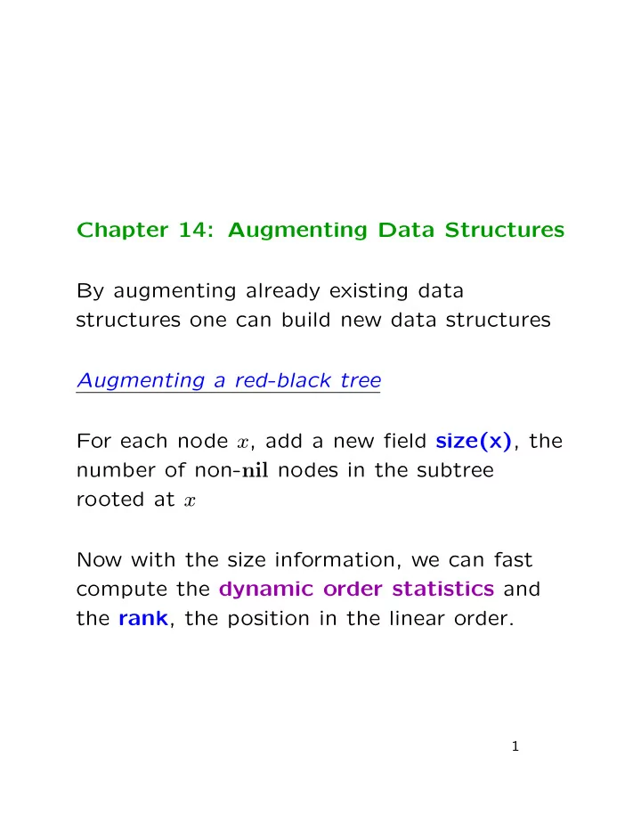
: red nodes : black nodes 2 1 6 2 3 1 1 1
What is the size of the root of the above RB-tree?
2
SLIDE 3 Selection To find the ith order statistics, run binary search. Let a and b be the size of the left child and that of the right child, respectively. Then we do the following
- If i = a + 1, the current node holds the
i-th o.s.
- If i < a + 1, search for the i-th o.s. in the
left subtree.
- If i > a + 1, search for the (i − a − 1)-st
- .s. in the right subtree.
What is the running time of this selection procedure?
3
SLIDE 4
a search for the i-th b the (i-a-1)-st search for a+b+1
4
SLIDE 5
Computing the Rank of a Given Node x
Rank(T, x)
1: m ← size[left[x]] + 1 2: y ← x 3: while y = root[T] do 4: { if right[p[y]] = x 5: then m ← m + size[left[p[y]]] + 1 6: y ← p[y] 7: } 8: Return(m)
5
SLIDE 6
b f d a e c x u
Here the rank of x is 1 + (c + 1) + (e + 1) = c + e + 3. What is the running time of rank?
6
SLIDE 7 Maintaining the Size Information During RB-Tree Operations
The size has to be changed for only one node:
- the left-child of the rotated node in the
case of right rotation and
- the right-child of the rotated node in the
case left rotation.
7
SLIDE 8
a+b+c+2
a+b+1
a a+b+c+2 c b
b+c+1
a b c
8
SLIDE 9
Climb up the tree from the actual point of insertion (respectively, deletion) all the way to the root. For each of the node that is encountered, and 1 to the size (respectively, subtract 1 from the size).
9
SLIDE 10 An Augmentation Strategy Augmenting a data structure can be broken into the following four steps:
- 1. choosing an underlying data structure,
- 2. determining what kind of additional
information should be maintained in the underlying data structure,
- 3. verify that the additional information
can be maintained during the execution
- f each basic modifying operation of the
underlying data structure, and
- 4. developing new operations.
10
SLIDE 11
The third step is easy for red-black trees. Theorem A Let f be a field that augments a red-black tree T of n nodes, and suppose that the f-value of a node x can be computed solely from the information stored at x and at its children. Then, maintaining the f-values of all nodes in T during insertion and deletion can be done in O(lg n) steps.
11
SLIDE 12 Proof Sketch Suppose that an operation has applied to an RB-tree T. Let T ′ the RB-tree after this operation. There is a downward path π in T ′ such that every node that has been “touched” (its
- r its children’s information has been
modified) is within distance three from the path. Thus, there are only O(log n) nodes for which the f-field has to be modified. So, store π and update the f-fields of all the nodes within distance 3 from the path in a bottom-up fashion.
12
SLIDE 13 An Illustrating Example: Interval trees For an interval i = [l, t], call l the low end and t the high end of i. The trichotomy of intervals For every pair of intervals i and j, exactly one
- f the following conditions holds:
- 1. i and j overlap
- 2. high[i] < low[j], i.e., j is to the right of i
- 3. high[j] < low[i], i.e., j is to the left of i
13
SLIDE 14 The Trichotomy b a c d
low[c]>high[b]
14
SLIDE 15 How can we maintain a dynamic set of closed intervals? Step 1: Underlying Data Structure Use the RB tree, where each node holds an
- interval. Use int[·] to refer to the interval.
Use lowint[·] as the key. Step 2: Additional Information At each node store as additional information the largest high end of the intervals in the subtree rooted at the node. Use max[·] to refer to this information.
15
SLIDE 16
Step 3: Maintaining max For all nodes x, max[x] is equal to max{high[int[x]], max[left[x]], max[right[x]]}. By the previous theorem, max can be maintained in O(lg n) steps.
16
SLIDE 17 Step 4: Developing New Operation The only new operation needed is searching for an interval that overlaps an interval i. Let T be the tree and i be the input. Then set x to the root and execute the following loop:
- If int[x] ∩ i = ∅, output int[x]. The search
is over. ;-)
- Otherwise, if x is a leaf, then output “no
intersecting intervals found.” :-(
- Otherwise, if x has a unique child, then
set x to the unique child.
- Otherwise, if the max[left[x]] ≥ low[i], then
set x to left[x].
- Otherwise, set x to right[x].
17
SLIDE 18
Theorem B The algorithm works correctly. Proof Call a subtree U good if it contains an interval overlapping i and bad otherwise. We have only to show that if (*) if T is good then Tx is good holds during the course of the algorithm. For initialization, the property (*) holds at the beginning of the search.
18
SLIDE 19 For the induction step, suppose that we are at non-leaf x and (*) holds. Suppose that T is good. Then by (*) Tx is good. Suppose that the interval at x does not intersect with
- i. Let y be the node that is visited at the
next round. We will show that Ty is good. Since the interval at x does not intersect with i, either the left subtree of x is good or the right subtree of x is good. This means that if there is only one child of x, then the unique child is good. Since y is this unique child (*) when x has only one child. So, assume that x has two children.
19
SLIDE 20 (Case 1) max[left[x]] ≥ low[i]: Here y = left[x]. (Case 1a) subtree(left[x]) is good: This implies Ty is good and T is good. So, (*) holds for y. (Case 1b) subtree(left[x]) is bad: Since max[left[x]] ≥ low[i] there is an interval to the right of i in the left subtree of x. This means that every interval in the right subtree is to the right of i. Thus, the right subtree is
- bad. So, both subtrees are bad, which is
- impossible. So, (Case 1b) never occurs.
(Case 2) max[left[x]] < low[i]: Here y = right[x]. Since max[left[x]] < low[i], there is no interval that intersects with i in the left subtree tree. So Ty is good.
20