17. Long Term Trends and Hurst Phenomena From ancient times the Nile - PowerPoint PPT Presentation

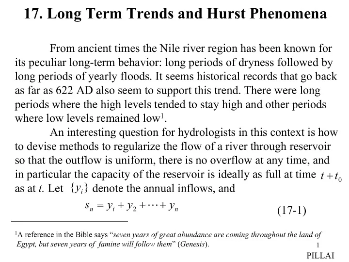
17. Long Term Trends and Hurst Phenomena From ancient times the Nile river region has been known for its peculiar long-term behavior: long periods of dryness followed by long periods of yearly floods. It seems historical records that go back as far as 622 AD also seem to support this trend. There were long periods where the high levels tended to stay high and other periods where low levels remained low 1 . An interesting question for hydrologists in this context is how to devise methods to regularize the flow of a river through reservoir so that the outflow is uniform, there is no overflow at any time, and t + in particular the capacity of the reservoir is ideally as full at time t 0 { y } as at t. Let denote the annual inflows, and i = + + + s y y � y (17-1) n i 2 n 1 A reference in the Bible says “ seven years of great abundance are coming throughout the land of Egypt, but seven years of famine will follow them ” ( Genesis ). 1 PILLAI

their cumulative inflow up to time n so that 1 s N ∑ = = y y N (17-2) N i N N = 1 i { y } represents the overall average over a period N . Note that may i as well represent the internet traffic at some specific local area y network and the average system load in some suitable time frame. N To study the long term behavior in such systems, define the “extermal” parameters = − u max { s n y }, (17-3) N n N ≤ ≤ 1 n N = − v min { s n y }, (17-4) N n N ≤ ≤ 1 n N as well as the sample variance 1 N ∑ = − 2 D ( y y ) . (17-5) N n N N = n 1 In this case = − 2 R u v (17-6) N N N PILLAI

defines the adjusted range statistic over the period N , and the dimen- sionless quantity − R u v = N N N (17-7) D D N N that represents the readjusted range statistic has been used extensively by hydrologists to investigate a variety of natural phenomena. R / D To understand the long term behavior of where N N = y i , i 1 , 2 , � N are independent identically distributed random µ σ variables with common mean and variance note that for large N 2 , by the strong law of large numbers n →  µ n σ d 2 s N ( n , ), (17-8) 2 N  → µ σ → µ y N ( , / ) d (17-9) N and  d → σ 2 D (17-10) 3 N PILLAI

n = Nt , with probability 1. Further with where 0 < t < 1, we have − µ   − µ s Nt s n =  → lim lim B ( t )  Nt  d n (17-11) σ σ N N → ∞ → ∞ N N where is the standard Brownian process with auto-correlation B ( t ) function given by min ( t 1 t , ). To make further progress note that 2 − = − µ − − µ s n y s n n ( y ) n N n N n = − µ − − µ ( s n ) ( s N ) (17-12) n N N so that − − µ − µ s ny s n n s N = −  → − < < d (17-13) n N n N ( ) B t tB (1), 0 t 1. σ σ σ N N N N Hence by the functional central limit theorem, using (17-3) and (17-4) we get 4 PILLAI

− u v  → − − − ≡ d N N max{ ( ) B t tB (1)} min{ ( ) B t tB (1)} Q , (17-14) N σ < < < < 0 t 1 0 t 1 where Q is a strictly positive random variable with finite variance. Together with (17-10) this gives − R u v →  → (17-15) d N N N N Q , σ D N a result due to Feller. Thus in the case of i.i.d. random variables the 1 / 2 R / D O ( N ). rescaled range statistic is of the order of It N N log( R / D ) follows that the plot of versus log N should be linear N N with slope H = 0.5 for independent and identically distributed observations. Slope=0.5 log( R / D ) N N ⋅ ⋅ ⋅ ⋅ ⋅ ⋅ ⋅ ⋅ ⋅ ⋅ ⋅ ⋅ ⋅ ⋅ ⋅ ⋅ ⋅ ⋅ ⋅ ⋅ ⋅⋅ ⋅ ⋅ ⋅ ⋅ 5 log N PILLAI

The hydrologist Harold Erwin Hurst (1951) generated tremendous interest when he published results based on water level data that he analyzed for regions of the Nile river which showed that ≈ Plots of versus log N are linear with slope log( R / D ) H 0 . 75 . N N According to Feller’s analysis this must be an anomaly if the flows are i.i.d. with finite second moment. The basic problem raised by Hurst was to identify circumstances > under which one may obtain an exponent for N in (17-15). H 1 / 2 The first positive result in this context was obtained by Mandelbrot and Van Ness (1968) who obtained under a strongly > H 1 / 2 dependent stationary Gaussian model. The Hurst effect appears for independent and non-stationary flows with finite second moment also. In particular, when an appropriate slow-trend is superimposed on a sequence of i.i.d. random variables the Hurst phenomenon reappears. To see this, we define the Hurst exponent fora data set to be H if 6 PILLAI

R  → → ∞ Q , N , d (17-16) N D N H N where Q is a nonzero real valued random variable. IID with slow Trend Let be a sequence of i.i.d. random variables with common mean { X } n µ σ g 2 and variance and be an arbitrary real valued function , n on the set of positive integers setting a deterministic trend, so that = + y x g (17-17) n n n represents the actual observations. Then the partial sum in (17-1) becomes n ∑ = + + + = + + + + s y y � y x x � x g n 1 2 n 1 2 n i = i 1 = + (17-18) n ( x g ) n n ∑ = n = g 1 / n g where represents the running mean of the slow trend. n i i 1 7 From (17-5) and (17-17), we obtain PILLAI

1 N ∑ = − 2 D ( y y ) N n N N = n 1 1 1 2 N N N ∑ ∑ ∑ = − + − + − − 2 2 ( x x ) ( g g ) ( x x )( g g ) n N n N n N n N N N N = = = n 1 n 1 n 1 1 2 N N (17-19) ∑ ∑ = σ + − + − − 2 2 ˆ ( g g ) ( x x )( g g ). X n N n N n N N N = = n 1 n 1 { x } Since are i.i.d. random variables, from (17-10) we get n σ  d → σ { g } 2 2 Further suppose that the deterministic sequence ˆ . n X ∑ = 1 N g = converges to a finite limit c . Then their Caesaro means g 1 n N N n also converges to c . Since 1 1 N N ∑ ∑ − = − − − 2 2 2 ( g g ) ( g c ) ( g c ) , (17-20) n N n N N N = = n 1 n 1 g n − g N − 2 2 ( c ) ( c ) applying the above argument to the sequence and we get (17-20) converges to zero. Similarly, since 8 PILLAI

1 1 N N ∑ ∑ − − = − µ − − − µ − ( x x )( g g ) ( x )( g c ) ( x )( g c ), n N n N n n N N N N = = n 1 n 1 (17-21) by Schwarz inequality, the first term becomes 2 1 1 1 N N N ∑ ∑ ∑ − µ − ≤ − µ − (17-22) 2 2 ( x )( g c ) ( x ) ( g c ) . n n n n N N N = = = n 1 n 1 n 1 ∑ = ∑ = N N − µ → σ − → 2 2 2 ( x ) ( g c ) 0 . 1 1 But and the Caesaro means n n N N n 1 n 1 Hence the first term (17-21) tends to zero as and so does the → ∞ N , second term there. Using these results in (17-19), we get → ⇒  → σ (17-23) d 2 g c D . n N To make further progress, observe that = − u max { s n g } N n N = − + − max { n ( x x ) n ( g g )} n N n N ≤ − + − max { n ( x x )} max { n ( g g )} 9 (17-24) n N n N PILLAI < < < < 0 n N 0 n N

and = − v min { s n g } N n N = − + − min { n ( x x ) n ( g g )} n N n N ≥ − + − min { n ( x x )} min { n ( g g )}. (17-25) n N n N < < < < 0 n N 0 n N Consequently, if we let = − − − (17-26) r max { n ( x x )} min { n ( x x )} N n N n N < < < < 0 n N 0 n N for the i.i.d. random variables, then from (17-6),(17-24) and (17-25) (17-26), we obtain = − ≤ + R u v r G (17-27) N N N N N where (17-28) = − − − G max { n ( g g )} min { n ( g g )} N n N n N < < < < 0 n N 0 n N From (17-24) – (17-25), we also obtain 10 PILLAI

≥ − + − u min { n ( x x )} max { n ( g g )}, (17-29) N n N n N < < < < 0 n N 0 n N ≤ − + − v max { n ( x x )} min { n ( g g )}, (17-30) N n N n N < < < < 0 n N 0 n N + ≥ + = + [use max {( x y )} max {( min x ) y } min ( x ) max ( y )] and hence i i i i i i i i i i i ≥ − R G r . (17-31) N N N From (17-27) and (17-31) we get the useful estimates − ≤ R G r , N N N (17-32) and − ≤ R r G . (17-33) N N N Since are i.i.d. random variables, using (17-15) in (17-26) we get { x } n r r → σ → N N Q , in probabilit y (17-34) σ ˆ 2 N N X a positive random variable, so that r N → N Q in probabilit y. (17-35) 11 σ PILLAI