15-112 Fundamentals of Programming Week 3 - Lecture 3: Efficiency - - PowerPoint PPT Presentation

June 2, 2016

15-112 Fundamentals of Programming

Week 3 - Lecture 3: Efficiency continued + Sets and dictionaries.

Measuring running time

• for strings: = number of characters

N

• for lists: = number of elements

N

• for ints: = number of digits

N > Running time is a function of . N > Look at worst-case scenario/input of length . N > Count algorithmic steps. > Ignore constant factors. (e.g. ) N 2 ≈ 3N 2 How to properly measure running time (use big Oh notation) > Input length/size denoted by (and sometimes by ) N n

Review

Number of times you need to divide N by 2 to reach 1. What is the big Oh notation used for? Upper bound a function by ignoring:

• constant factors
• small N.

ignore small order additive terms. Give 2 definitions of log2 N The number k that satisfies . 2k = N

Review

Big-Oh is the right level of abstraction! “Sweet spot”

• coarse enough to suppress details like

programming language, compiler, architecture,…

• sharp enough to make comparisons between

different algorithmic approaches. is analogous to “too many significant figures”. 8N 2 − 3n + 84 O(N 2)

Review

1010n3 is O(n3)? n10000 is O(1.1n)? n is O(n2)? n3 is O(2n)? 100n log2 n is O(n)? 1000 log2 n is O(√n)? 1000 log2 n is O(n0.00000001)? Yes Yes Yes Yes No Yes Yes Does the base of the log matter?

When we ask “what is the running time…” you must give the tight bound!

logb n = logc n logc b

constant

Review

Constant:

O(1)

Logarithmic:

O(log n)

Square-root:

O(√n) = O(n0.5)

Linear:

O(n)

Loglinear:

O(n log n)

Quadratic:

O(n2)

Exponential:

O(kn)

Polynomial:

O(nk)

Review

log n <<< √n << n < n log n << n2 << n3 <<< 2n <<< 3n

Review

Running time of Bubble Sort: Running time of Selection Sort: Why is Bubble Sort slower than Selection Sort in practice? Running time of Linear Search: Running time of Binary Search: O(N) O(log N) O(N 2) O(N 2)

Review: selection sort code

2 8 7 99 4 5

start len(a) - 1

Find the min position from start to len(a) - 1

min position

Swap elements in min position and start Increment start Repeat Selection sort snapshot:

Review: selection sort code

2 8 7 99 4 5

start len(a) - 1

Find the min position from start to len(a) - 1

min position

Swap elements in min position and start for start = 0 to len(a)-1: Selection sort snapshot:

Review: selection sort code

def selectionSort(a): Find the min position from start to len(a) - 1 Swap elements in min position and start

2 8 7 99 4 5

start len(a) - 1 min position for start = 0 to len(a)-1: for start in range(len(a)): currentMinIndex = start for i in range(start, len(a)): if(a[i] < a[currentMinIndex]): currentMinIndex = i (a[currentMinIndex], a[start]) = (a[start], a[currentMinIndex])

Review: bubble sort code

repeat until no more swaps: for i = 0 to end: if a[i] > a[i+1], swap a[i] and a[i+1] decrement end Bubble sort snapshot 4 7 5 8 99 2

end a[i] a[i+1]

Review: bubble sort code

4 7 5 8 99 2

end a[i] a[i+1] repeat until no more swaps: for i = 0 to end: if a[i] > a[i+1], swap a[i] and a[i+1] decrement end def bubbleSort(a): swapped = True end = len(a)-1 while(swapped): swapped = False for i in range(end): if(a[i] > a[i+1]): (a[i], a[i+1]) = (a[i+1], a[i]) swapped = True end -= 1

Review

You have an algorithm with running time . O(N) If we double the input size, by what factor does the running time increase? If we quadruple the input size, by what factor does the running time increase? If we double the input size, by what factor does the running time increase? If we quadruple the input size, by what factor does the running time increase? You have an algorithm with running time . O(N 2)

Review

Give an example of an algorithm that requires exponential time. Exhaustive search for the Subset Sum Problem. Can you find a polynomial time algorithm for Subset Sum? To search for an element in a list, it is better to:

• sort the list, then do binary search, or
• do a linear search?

The Plan > Measuring running time when the input is an int > Merge sort > Efficient data structures: sets and dictionaries

Merge Sort: Merge

Merge The key subroutine/helper function: merge(a, b) Input: two sorted lists a and b Output: a and b merged into a single list, all sorted. Turns out we can do this pretty efficiently. And that turns out to be quite useful!

Merge Sort: Merge Algorithm

Merge 8 9 11 1 3 12 4 16 15 a = b = c = Main idea: min(c) = min(min(a), min(b))

Merge Sort: Merge Algorithm

Merge 8 9 11 1 3 12 4 16 15 a = b = c = Main idea: min(c) = min(min(a), min(b)) 1

Merge Sort: Merge Algorithm

Merge 8 9 11 1 3 12 4 16 15 a = b = c = Main idea: min(c) = min(min(a), min(b)) 1

Merge Sort: Merge Algorithm

Merge 8 9 11 1 3 12 4 16 15 a = b = c = Main idea: min(c) = min(min(a), min(b)) 1 3

Merge Sort: Merge Algorithm

Merge 8 9 11 1 3 12 4 16 15 a = b = c = Main idea: min(c) = min(min(a), min(b)) 1 3

Merge Sort: Merge Algorithm

Merge 8 9 11 1 3 12 4 16 15 a = b = c = Main idea: min(c) = min(min(a), min(b)) 1 3 4

Merge Sort: Merge Algorithm

Merge 8 9 11 1 3 12 4 16 15 a = b = c = Main idea: min(c) = min(min(a), min(b)) 1 3 4

Merge Sort: Merge Algorithm

Merge 8 9 11 1 3 12 4 16 15 a = b = c = Main idea: min(c) = min(min(a), min(b)) 1 3 4 8

Merge Sort: Merge Algorithm

Merge 8 9 11 1 3 12 4 16 15 a = b = c = Main idea: min(c) = min(min(a), min(b)) 1 3 4 8

Merge Sort: Merge Algorithm

Merge 8 9 11 1 3 12 4 16 15 a = b = c = Main idea: min(c) = min(min(a), min(b)) 1 3 4 8 9

Merge Sort: Merge Algorithm

Merge 8 9 11 1 3 12 4 16 15 a = b = c = Main idea: min(c) = min(min(a), min(b)) 1 3 4 8 9

Merge Sort: Merge Algorithm

Merge 8 9 11 1 3 12 4 16 15 a = b = c = Main idea: min(c) = min(min(a), min(b)) 1 3 4 8 9 11

Merge Sort: Merge Algorithm

Merge 8 9 11 1 3 12 4 16 15 a = b = c = Main idea: min(c) = min(min(a), min(b)) 1 3 4 8 9 11

Merge Sort: Merge Algorithm

Merge 8 9 11 1 3 12 4 16 15 a = b = c = Main idea: min(c) = min(min(a), min(b)) 1 3 4 8 9 11 12

Merge Sort: Merge Algorithm

Merge 8 9 11 1 3 12 4 16 15 a = b = c = Main idea: min(c) = min(min(a), min(b)) 1 3 4 8 9 11 12

Merge Sort: Merge Algorithm

Merge 8 9 11 1 3 12 4 16 15 a = b = c = Main idea: min(c) = min(min(a), min(b)) 1 3 4 8 9 11 12 15

Merge Sort: Merge Algorithm

Merge 8 9 11 1 3 12 4 16 15 a = b = c = Main idea: min(c) = min(min(a), min(b)) 1 3 4 8 9 11 12 15

Merge Sort: Merge Algorithm

Merge 8 9 11 1 3 12 4 16 15 a = b = c = Main idea: min(c) = min(min(a), min(b)) 1 3 4 8 9 11 12 15 16

Merge Sort: Merge Algorithm

Merge 8 9 11 1 3 12 4 16 15 a = b = c = Main idea: min(c) = min(min(a), min(b)) 1 3 4 8 9 11 12 15 16

Merge Sort: Merge Running Time

Merge 8 9 11 1 3 12 4 16 15 a = b = c = Running time? 1 3 4 8 9 11 12 15 16 N = len(a) + len(b) O(N) # steps:

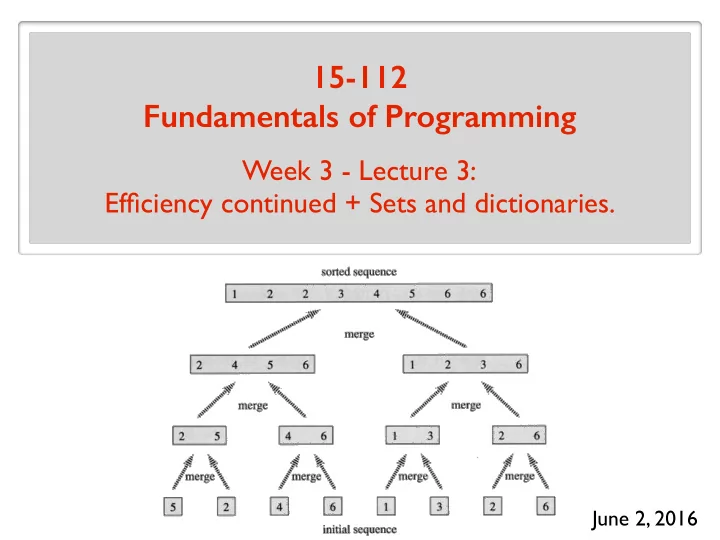
Merge Sort: Algorithm

merge merge merge merge merge merge Merge Sort

Merge Sort: Running Time

Total: O(N log N) O(N) O(N) O(N) O(log N) levels

The Plan > Measuring running time when the input is an int > Merge sort > Efficient data structures: sets and dictionaries

Integer inputs

def isPrime(n): if (n < 2): return False for factor in range(2, n): if (n % factor == 0): return False return True

Simplifying assumption in 15-112: Arithmetic operations take constant time.

Integer inputs

def isPrime(n): if (n < 2): return False for factor in range(2, n): if (n % factor == 0): return False return True

What is the input length? = number of digits in n ~ log10 n

Integer Inputs

def isPrime(m): if (m < 2): return False for factor in range(2, m): if (m % factor == 0): return False return True

What is the input length? = number of digits in m ~ log10 m What is the running time? (actually because it is in binary)

log2 m

So N ∼ log2 m O(m) O(2N) = i.e., m ∼ 2N

Integer Inputs

def fasterIsPrime(m): if (m < 2): return False maxFactor = int(round(m**0.5)) for factor in range(3, maxFactor+1): if (m % factor == 0): return False return True

What is the running time? O(2N/2)

Not feasible when . N = 2048

isPrime

Amazing result from 2002: There is a polynomial-time algorithm for primality testing. Agrawal, Kayal, Saxena undergraduate students at the time However, best known implementation is ~ time. O(N 6)

isPrime

So that’s not what we use in practice. The running time is ~ . O(N 2) It is a randomized algorithm with a tiny error probability. 1/2300 (say ) Everyone uses the Miller-Rabin algorithm (1975).

CMU Professor

The Plan > Measuring running time when the input is an int > Merge sort > Efficient data structures: sets and dictionaries

Tangent

Can we cheat exponential time?

What is a data structure?

A data structure allows you to store and maintain a collection of data. It should support basic operations like:

• add an element to the data structure
• remove an element from the data structure
• find an element in the data structure

…

What is a data structure?

A list is a data structure. It supports basic operations:

• append( )
• remove( )
• in operator, index( )

… O(1) O(N) O(N) One could potentially come up with a different structure which has different running times for basic operations.

Motivating example

Sorting a list of numbers. What if I know all the numbers are less than 1 million. … m 1 Put number m at index m. Create a list of size 1 million. Solution: What is the running time for searching for an element? O(1)

Motivating example

The sweet idea: Connecting value to index. … m 1

Motivating example

What if the numbers are not bounded by a million? What if you want to store strings rather than numbers? Questions

Extending the sweet idea

Storing a collection of strings? … Start with a certain size list (e.g. 100) s h(s) Pick a function h that maps strings to numbers. h is called a hash function. Store s at index h(s) mod (size of list) s mod (size of list)

Extending the sweet idea

Potential Problems Collision: two strings map to the same index List fills up Fixes The hash function should be “random” so that the likelihood of collision is not high. When buckets get large (say more than 10), resize and rehash: pick a larger list, rehash everything Store multiple values at one index (bucket) (e.g. use 2d list) HASH TABLE

Extending the sweet idea

What did we gain: Basic operations add, remove, find/search super fast (sometimes (infrequently) we need to resize/rehash) What did we lose: No order No mutable elements Repetitions are not good

Sets

Introducing sets

• supports basic operations like:

s.add(x), s.remove(x), s.union(t), s.intersection(t) x in s Sets:

• a non-sequential (unordered) collection of objects
• no repetitions allowed
• look up by object’s value
• immutable elements
• finding a value is super efficient

Creating a set

s = set([2, 4, 8]) s = set([“hello”, 2, True, 3.14]) s = set([2, 2, 4, 8]) s = set([2, 4, [8]]) # Error

(sets are mutable, but its elements must be immutable.)

s = set(“hello”) s = set((2, 4, 8)) s = set(range(10)) s = set() # {8, 2, 4} # {“hello”, True, 2, 3.14} # {8, 2, 4} # {‘e’, ‘h’, ‘l’, ‘o’} # {8, 2, 4} # {0, 1, 2, 3, 4, 5, 6, 7, 8, 9}

Set methods

s.copy() s.union(t), s.intersection(t), s.difference(t), s.symmetric_difference(t) s.add(x), s.remove(x), s.discard(x)

Returns a new set (non-destructive): Modifies s (destructive):

s.pop(), s.clear() s.update(t), s.intersection_update(t), s.difference_update(t), s.symmetric_difference_update(t)

Other:

s.issubset(t), s.issuperset(t) s t s t

The advantage over lists

s = set() for x in range(10000): s.add(x) print(5000 in s) print(-1 not in s) s.remove(100) # Super fast # Super fast # Super fast

Essentially O(1)

Example: checking for duplicates

Given a list, want to check if there is any element appearing more than once.

Dictionaries (Maps)

Dictionaries / maps

Lists:

• a sequential collection of objects

Dictionaries:

• a non-sequential (unordered) collection of objects
• a more flexible look up by keys
• can do look up by index (the position in the collection)

Dictionaries / maps

“slkj2” “4@4s” “as43” “9idj” 1 2 3 4

List

a = [None]*5 a[0] = “slkj2” a[1] = “4@4s” a[2] = “as43” a[3] = “9idj” a[4] = “9idj”

keys values

Dictionaries / maps

d = dict() d[“alice”] = “slkj2” d[“bob”] = “4@4s” d[“charlie”] = “as43” d[“david”] = “9idj” d[“eve”] = “9idj”

keys values

“alice” “bob” “charlie” “david” “eve” “slkj2” “4@4s” “as43” “9idj”

HASH TABLE

• hash using the key
• store (key, value) pair
• unordered
• values are mutable
• keys form a set

(immutable, no repetition)

Properties:

Dictionaries / maps

users = dict() users[“alice”] = “sl@3” users[“bob”] = “#$ks” users[“charlie”] = “slk92” users = {“alice”: “sl@3”, “bob”: “#$ks”, “charlie”: “slk92”} users = [(“alice”, “sl@3”), (“bob”, “#$ks”), (“charlie”, “#242”)] users = dict(users)

Creating dictionaries

Dictionaries / maps

for key in users: print(key, d[key]) print(users[“frank”]) print(users.get(“frank”)) print(users.get(“frank”, 0)) Error # prints None # prints 0 users = {“alice”: “sl@3”, “bob”: “#$ks”, “charlie”: “slk92”}

Example: Find most frequent element

Input: a list of integers Output: the most frequent element in the list 1 2 3 count elements

• f the list

Exercise: Write the code.