13-Feb-19 Economics of Power Generation Economics of Power - - PowerPoint PPT Presentation

13-Feb-19 1

Economics of Power Generation

• In whatever we do, energy plays an important role.
• There can be numerous energy resources.
• Choice of a particular energy resource depends on availability of energy resource and

its life cycle cost.

• For example, for generation of electricity, there are two options: centralized or local

decentralized.

• For centralized production lots of T&D infrastructure is required, there are advantages
• f ‘Economy of Scale’ and upkeep and maintenance is easy.
• For local centralized production, there are no T&D hassles but there is O&M

requirements.

• To choose between the two, economics of power generation needs to be assessed.

Economics of Power Generation

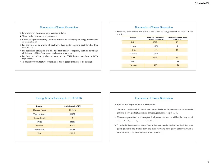
• Electricity consumption per capita is the index of living standard of people of that

country.

Country Electricity Consumption (kWh) per capita in 2018 Human Development Index (HDI) 2018

USA 12071 13 China 4475 86 Japan 7371 19 Norway 26006 1 UAE 16195 34 India 1122 130 Pakistan 405 150

Energy Mix in India (up to 31.10.2018)

Resource Installed capacity (MW)

Thermal (coal) 195993 Thermal (gas) 24937 Thermal (oil) 838 Hydro 45487 Nuclear 6780 Renewable 72013

Total 346048

Economics of Power Generation

• India has fifth largest coal reserves in the world.
• The problem with fossil fuel based power generation is scarcity concerns and environmental

concerns (1 kWh electricity generated from coal, produces 0.94 kg of CO2) .

• With current production and consumption level, proven coal reserves will last for 110 years, oil

reserves for 50 years and gas reserves for 52 years.

• To maintain ‘intergeneration equity’ there is dire need to reduce reliance on fossil fuel based

power generation and promote more and more renewable based power generation which is sustainable and at the same time environment friendly.

13-Feb-19 2

CO2 Emissions due to Electricity used in an Electric Geyser for a Single Bath

Details Energy Requirement Form of Energy Additional Parameters Energy required to heat 30 kg water from 15oC- 40oC (30 kg) (4.2 kJ/kgoC) (40-15)oC = 3150 kJ Useful Energy

• Sp. Heat of water

= 4.2 kJ/kgoC Electricity used by electric geyser 3150 / 0.95 = 3316 kJ Final Energy Efficiency of electric geyser = 0.95 Electricity dispatched from the power plant 3316 / (1- 0.15) = 3901 kJ Secondary Energy Transmission and Distribution losses of electricity = 15% Amount of energy contributed by coal at the thermal power plant 3901 / 0.4 = 9752 kJ Primary Energy Overall efficiency of coal thermal power plant = 40% Amount of Coal used 9752 kJ / 20000 kJ/kg = 0.488 kg

• Lower heating value of Coal

= 20 MJ / kg Amount of CO2 released (0.488) (0.6) (44/12) (100) = 1.073 kg

• Carbon fraction in Coal = 0.6

Fraction of carbon oxidized = 1.0

Carbon Dioxide Mitigation Potential of Domestic Solar Water Heating System

Rated Capacity of Domestic Solar Water Heating System (SWHS) = 200 litres /day Initial temperature of water = 15oC Design delivery temperature of water = 60oC Annual Capacity Utilization Factor for Domestic SWHS = 0.75 Density of water = 1000 kg / m3 Annual useful energy delivered by the domestic SWHS = (0.75) (365 days/year) (200 kg/day) (4.2 kJ/kgoC) (60 – 15)oC = 10347750 kJ per year

Carbon Dioxide Mitigation Potential of Domestic Solar Water Heating System

It is assumed that prior to the installation of the domestic SWHS, the household uses an electric geyser (efficiency of electricity utilization = 95%) with the electricity being produced in a coal thermal power plant. Transmission and Distribution losses of electricity = 15% Overall efficiency of coal utilization in coal thermal power plant = 40% Carbon fraction in coal used = 0.60 Lower heating value of coal used = 20 MJ / kg Annual amount of coal saved due to use of domestic SWHS Amount of CO2 emissions likely to be mitigated annually = (1601.819) (0.6) (44/12) = 3524 kg of CO2 = 3.5 tonnes of CO2

coal

• f

kg 1601 ) kg / kJ 20000 )( 40 . )( 15 . 1 )( 95 . ( kJ 10347750   

Economics of Power Generation

Technology Capital Cost ($/kW) Operating Cost ($/kWh) Coal-fired combustion turbine $500 — $1,000 0.20 — 0.04 Natural gas combustion turbine $400 — $800 0.04 — 0.10 Coal gasification combined-cycle (IGCC) $1,000 — $1,500 0.04 — 0.08 Natural gas combined-cycle $600 — $1,200 0.04 — 0.10 Wind turbine (includes offshore wind) $1,200 — $5,000 Less than 0.01 Nuclear $1,200 — $5,000 0.02 — 0.05 Photovoltaic Solar $4,500 and up Less than 0.01 Hydroelectric $1,200 — $5,000 Less than 0.01

13-Feb-19 3

Economics of Power Generation

When planning a power plant, two basic parameters to be decided are:

• Total installed capacity
• Size of the generating unit

Economics of Power Generation

Total installed capacity can be determined from:

• Maximum demand
• Growth of demand
• Reserve capacity required

Economics of Power Generation

Size of generating unit depends on:

• Variation of load during 24 hours
• Maximum startup and shut down time
• Maintenance programme
• Total capacity connected to the grid
• Plant efficiency versus size of unit
• Prize and space demand per kW versus size of unit

Load Curves for a Power Plant

• The Load Curve is a Graph, which represents load on the generation station (the load is

in kW/MW) recorded at the interval of half hour or hour (time)

• It is a curve which is drawn between loads versus time in sequential order. They are

drawn on daily basis data, weekly or monthly basis data.

13-Feb-19 4

Load Curves for a Power Plant

The Load Curve gives following Information:

• The daily load curve shows the variation of load on the power station during different

hours of the day.

• The area under the daily load curve gives the number of unit generated in the day. Unit

generated/day= Area (in kWh) under daily load curve.

• The highest point on the daily load curve represents the maximum demand on the

station on that day.

• The area under the daily load curve divided by the total number of hours gives the

average load on the station in that day.

hours 24 curve load daily under the kWh) (in Area load Average 

Load Duration Curves

• When the load elements of a load curve are arranged in the order of descending

magnitudes, the curve thus obtained is called a load duration curve.

• The load duration curve is obtained from the same data as load curve but the ordinate

representing the maximum load is represented to the left and the decreasing loads are represented to the right in the descending order.

Load Duration Curves

The load duration curve provides following useful information:

• The load duration curve readily shows the number of hours during which the given load

has prevailed.

• The area under daily load duration curve (in kWh) will give the units generated on that

day.

• The load duration curve, helps to give information about annual load duration curve.

Factors affecting cost of generation

• Load factor
• Capacity factor
• Reserve factor
• Plant use factor
• Demand factor
• Diversity factor

13-Feb-19 5

Factors affecting cost of generation

• Load factor:

The ratio of number of units actually generated in a given period to number of units which could have been generated with the same maximum demands is called as load factor for the station. OR The Ratio of Average Load to the Maximum Demand during a given period is known as load factor. 8760 kW year an in generated kWh factor Load load Peak load Average factor Load

max 

 

Plant Load Factor

• Plant Load factor:

It is a measure of average capacity utilization. If the PLF is affected by non-availability of fuel, maintenance shut-down, unplanned break down and no offtake (as consumption pattern fluctuates lower in nights), the generation has to be adjusted. A power (electricity) storage is not feasible. Generation of power is controlled to match the offtake. For any such duration, a power plant generates below its full capacity. To that extent it is a capacity loss.

• Higher the load factor, greater is the total output.
• A power plant shall be less efficient at lower load factors
• A high load factor means fixed costs are spread over more kWh of output.

Plant Load Factor in India

• Plant Load factor:

Year National PLF (Coal) (In percentage) NTPC PLF (Coal) (In percentage)

2007-08 78.5 92.2 2008-09 77.2 91.1 2009-10 77.5 90.8 2010-11 75.1 88.3 2011-12 73.3 85.0 2012-13 70.0 83.0 2013-14 64.62 79.14

Factors affecting cost of generation

• Capacity factor

The Plant Capacity Factor is the ratio of average demand on the Power Station divided by the maximum installed capacity of the power station. OR It is the ratio of actual energy produced to the maximum possible energy that could have been produced during a given period. 8760 kW kWh factor Capacity plant the

• f

capacity Rated load Average factor Capacity

installed generated

  

13-Feb-19 6

Factors affecting cost of generation

• Reserve factor

It is the ratio of installed capacity and maximum demand OR In other words, the difference between load factor and capacity factor is an indication of Reserve capacity

kW kW factor Reserve

maximum installed



Factors affecting cost of generation

• Plant use factor
• It is the ratio of kWh generated to the product of plant capacity and the number of hours

for which the plant was in operation.

• Plant use factor indicated how much is the plant capacity utilized, but it does not

indicate the time for which the plant remained idle.

• peration
• f

hours kW kWh factor use Plant

installed generated

 

Factors affecting cost of generation

• Demand factor
• It is the ratio of maximum demand to the total connected load.
• It is always less than unity.
• It will always change with time of use and will not remain constant.
• Connected load is always known so it will be easy to calculate maximum demand if

demand factor for a certain supply is known at different time interval.

load connected Total demand Maximum factor Demand 

Factors affecting cost of generation

• Diversity factor
• This term is used to measure time distribution of maximum demand of similar type of

consumer.

• It is the ratio of sum of maximum demand of individual consumer and simultaneous

maximum demand of the whole group.

• This is used to estimate total load required for a facility or to size a transformer

system the

• f

load peak Actual demand consumer individual

• f

Sum factor Diversity 

13-Feb-19 7

Factors affecting cost of generation

Feeder – 1 Demand load = 2000*0.7 = 1400 kVA ; Feeder – 2 Demand load = 1500*0.6 = 900 kVA ; Feeder – 3 Demand load = 1000*0.5 = 500 kVA ; Total Demand load = 2800 kVA ; Transformer demand load = 2800/ Diversity factor = 2545 kVA; Without Demand and Diversity factor, it would be 2000+1500+1000 = 4500 kVA

Main Transformer Diversity factor = 1.1 Feeder – 1 2000 kV A Demand factor = 0.7 Feeder – 2 1500 kV A Demand factor = 0.6 Feeder – 3 1000 kV A Demand factor = 0.5

Economics of Power Generation

• Larger the unit size, less is the cost of electricity produced. Hence larger units are more

economical than smaller ones.

• A reserve factor of 1.2 to 1.25 is found to be satisfactory.
• For economic operation of the generation unit and also for planning of tariffs, it is

useful to construct load duration curves for typical days that includes power demand at different intervals of time.

Economics of Power Generation

Loads can be:

• Residential
• Industrial
• Commercial
• Municipal
• Irrigation and traction

Economics of Power Generation

13-Feb-19 8

Economics of Power Generation

The area under the annual load duration curve represents total energy supplied by the

• utility. It is divided into three parts:
• Base load
• Intermediate load
• Peak load

Demand never falls below the base load and it operates for 100% of the time. The peak load occurs for 15% of the time and intermediate load represents remaining load regions.

Economics of Power Generation

By judicious combination of all three types of generation, maximum economy can be achieved.

• Base load plant should be run at high load factor.
• Peak load plant should be of smaller capacity to reduce cost of generation.
• It could be a gas turbine, pumped hydro station or diesel engine depending on size and

scope of availability.

Location of a Power Plant

Following factors needs to be considered:

• Availability of cooling water
• Availability of fuel
• Distance from utility
• Cost of land (space for extension, workshop, storage yard etc.)
• Characteristics of soil
• Ecological considerations
• Disposal of ash (with coal fired stations)
• Accommodation of staff
• Rail and road connections
• Security considerations

Power Plant Economics

Power plant should provide a reliable electricity supply at minimum cost to the consumer. The cost per kWh is determined by:

• Fixed cost (Interest, depreciation, insurance, taxes on the capital invested) including

cost of land

• O&M cost including salaries and wages, repairs and miscellaneous expenses
• Fuel cost depending on amount of electricity generated
• Net kWh generated

Total annual cost Ct is given by:

f c t

C M) R (W C 100 T D I C        

13-Feb-19 9

Power Plant Economics

Net electricity produced is given by:

Is this the cost of electricity to the consumers???????

In order to calculate electricity cost to a consumer, in addition to the production cost (fixed cost, O&M and fuel cost), Transmission and distribution cost, administrative expenses and return on investment should also be considered.

n) consumptio Aux.

• (1

C.F. 8760 kW kWh

installed net

   

generation y electricit net cost annual Total ty Electrici

• f

Cost 

Time Value of Money

• Money has a time value – its value changes (usually increases) with time.
• Money can be invested to earn more money between two intervals of time
• Money available at an earlier point in time is more valuable than the same amount

available later.

• Purchasing power of money (currency) may change between two time intervals

Time Value of Money

If it is assumed that the time rate of change of the value of money is constant for a specific duration of time, then:

• A particular factor could be used to describe the time value of money and thus to

determine equivalent value of a certain amount of cash flow at a certain point in time at some other point in time.

• Discount Rate (d) is often used for this purpose. It is expressed as a fraction.
• A value ‘d’ ’ of the discount rate implies that a certain amount P at present (t=0) would

be equivalent to an amount P(1+d) after one year with time value of money considerations.

Time Value of Money

Discount rate (d) is given by: Where r is the interest rate and I is Inflation rate. If r = 15% and I = 5% then discount rate d shall be 9.5%

I 1 I

• r

d  

13-Feb-19 10

2 4 6 8 10 12 14 16 18 20 1970 1975 1980 1985 1990 1995 2000 2005 2010 2015 2020 Interest Rate (%) Years India Japan Germany United States China Sweden

Time Trend of Interest Rate

• 1970 - 2017

Source: World Bank, 2018. http://www.data.worldbank.org/

Time Trend of Interest Rate

• 1970 - 2017

2 4 6 8 10 12 14 16 18 20 2008 2010 2012 2014 2016 2018 Interest Rate (%) Years India Japan Germany United States China Sweden

Time Trend of Inflation Rate

• 1970 - 2017
• 10
• 5

5 10 15 20 25 30 35 1955 1960 1965 1970 1975 1980 1985 1990 1995 2000 2005 2010 2015 2020 Inflation (%) Years Japan Germany USA India China Sweden

Source: World Bank, 2018. http://www.data.worldbank.org/

Time Trend of Inflation Rate

• 1970 - 2017
• 10
• 5

5 10 15 2008 2010 2012 2014 2016 2018 Inflation (%) Years Japan Germany USA India China Sweden

13-Feb-19 11

Formulae based on Time Value of Money Need for considering Time Value of Money

• Need for evaluating levelized cost of electricity of electricity generation option
• For finding amount to be saved annually for scheduled change of equipments. For

example change of batteries every 5 years in stand alone PV plant

• For finding Net Present value of any investment proposed.
• For finding benefit to cost ratio of a project
• For taking decision on economic viability of a project

Numerical Problem

• 1. It is proposed to replace an electric geyser with efficiency of 95% by a 100 lpd SWHS

to raise the temperature of water from 10°C to 60°C for a city like Ajmer having 300 sunny days a year. If price of electricity is Rs. 5 per kWh, what will be the annual monetary saving? Is the project worth investing if its cost is Rs. 25000?

Numerical Problem

Solution:

Useful energy delivered by geyser per day = Since 1 kWh = 3600 kJ therefore 22105 kJ = 6.14 kWh per day Further no. of units saved annually = 6.14 * 300 (number of sunny days) = 1842 kWh Monetary saving @Rs. 5 per kWh = 1842*5 = Rs. 9210 Assuming annual maintenance cost as Rs. 1000, Net annual monetary saving = Rs. 8210 Assuming price of electricity, annual output of SWHS and maintenance cost over the entire useful life as constant, Equivalent present value of life cycle monetary savings (assuming n = 25 years and d = 10%) Since present investment is Rs. 25000 therefore the project is worth investing.

kJ 22105 0.95 10)

• (60

4.2 100 t mc

geyser p

     

74522 Rs. d) d(1 1 d) A(1 P

n n

    

13-Feb-19 12

What if number of sunny days reduces to 100 per year?

Depreciation

• The power plant and associated equipments at the power plant will have a certain useful

life

• After years of use, the equipment loses its efficiency or become obsolete and needs

replacement

• Sometimes, equipment may have to be changed even when fairly new, if more efficient

equipment has come into the market

To enable this to be done when necessary, some money is put aside annually and is known as ‘Depreciation Fund’

Depreciation

The two methods of accumulating depreciation fund are: a) Straight line method b) Sinking fund method

Depreciation

The two methods of accumulating depreciation fund are: a) Straight line method Depreciation charge per year = (Initial Value – salvage Value) / useful life b) Sinking fund method Amount that should be set aside annually 1

• d)

(1 d value) salvage

• value

(initial

n

  