10/04/2018 Definitions A schedule is said to be feasible if it - PDF document

10/04/2018 Definitions A schedule  is said to be feasible if it satisfies a set of constraints. A task set  is said to be feasible , if there exists an algorithm that generates a feasible schedule for  . A task set  is said to be schedulable with an algorithm A, if A generates a feasible schedule. Examples of constraints • Timing constraints: activation, period, deadline, jitter. • Precedence: order of execution between tasks. • Resources: synchronization for mutual exclusion. 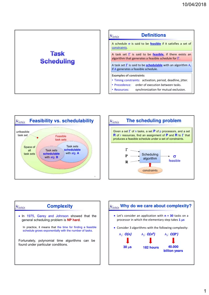The scheduling problem Feasibility vs. schedulability Given a set  of n tasks, a set P of p processors, and a set unfeasible R of r resources, find an assignment of P and R to  that task set Feasible produces a feasible schedule under a set of constraints. task sets Task sets Space of Space of  all Task sets schedulable with alg. A task sets schedulable Scheduling  P with alg. B algorithm feasible R constraints 3 Complexity Why do we care about complexity?  Let’s consider an application with n = 30 tasks on a  In 1975, Garey and Johnson showed that the processor in which the elementary step takes 1  s general scheduling problem is NP hard . In practice, it means that the time for finding a feasible  Consider 3 algorithms with the following complexity: schedule grows exponentially with the number of tasks. A 1 : O(n) O( ) A 2 : O(n 8 ) O( 8 ) A 3 : O(8 n ) O(8 ) Fortunately, polynomial time algorithms can be found under particular conditions. 30  s 40.000 182 hours billion years 1

10/04/2018 Simplifying assumptions Task set assumptions We consider algorithms for different types of tasks:  Single processor  Single-job tasks (one shot)  Homogeneous task sets tasks with a single activation (not recurrent)  Fully preemptive tasks  Periodic tasks  Periodic tasks  Simultaneous activations recurrent tasks regularly activated by a timer (each task potentially generates infinite jobs)  No precedence constraints  Aperiodic/Sporadic tasks  No resource constraints recurrent tasks irregularly activated by events (each task potentially generates infinite jobs)  Mixed task sets Classical scheduling policies First Come First Served It assigns the CPU to tasks based on their arrival  First Come First Served times (intrinsically non preemptive):  Shortest Job First Ready queue  Priority Scheduling  Priority Scheduling  4  3  2  1 CPU  Round Robin   1  2  3  4 Not suited for real-time systems t a 1 a 2 a 3 a 4 s 2 s 3 s 4 f 4 First Come First Served Shortest Job First (SJF) ‐ Very unpredictable It selects the ready task with the shortest response times strongly depend on task arrivals: computation time. a 1 a 2 a 3  Static (C i is a constant parameter) R 1 = 20 R 2 = 26 R 3 = 26  1  2  3  It can be used on line or off ‐ line t 0 4 8 12 16 20 24 28 32 a 3 a 2 a 1  Can be preemptive or non preemptive R 1 = 26 R 2 = 8 R 3 = 2  3  2  1  It minimizes the average response time t 0 4 8 12 16 20 24 28 32 11 12 2

10/04/2018 SJF - Optimality SJF - Optimality  SJF    ’  ’’  * L S . . .  ’      . . .  R (  ( ) ( ') ( ' ' ) *) S L R R R t t r 0 f S ’ < f L f L ’ = f S  * =  SJF f S ’ + f L ’  f S + f L R  ( ) is the minimum response time SJF 1 1 n n achievable by any algorithm          ( ') ( ' ) ( ) ( ) R f r f r R i i i i n n   1 1 i i 13 14 Is SJF suited for Real-Time? Priority Scheduling  Each task has a priority P i , typically P i  [0, 255] ‐ It is not optimal in the sense of feasibility  The task with the highest priority is selected for d 1 d 2 d 3 A  SJF feasible execution.  2  2  3  3  1  1  Tasks with the same priority are served FCFS  T k t ith th i it d FCFS 0 4 8 12 16 20 24 28 32 d 1 d 2 d 3 p i  1/C i  SJF not feasible SJF NOTE:  3  2  1 p i  1/a i  FCFS t 0 4 8 12 16 20 24 28 32 15 16 Priority Scheduling Round Robin The ready queue is served with FCFS, but ...  Problem: starvation ‐ Each task  i cannot execute for more than Q low priority tasks may experience long delays due to the preemption of high priority tasks. time units (Q = time quantum). ‐ When Q expires,  i is put back in the queue. When Q expires,  i is put back in the queue.  A possible solution: aging READY queue priority increases with waiting time CPU Q expired 17 18 3

10/04/2018 Round Robin Round Robin n = number of task in the system ‐ if Q > max(C i ) then RR  FCFS nQ nQ ‐ if Q  context switch time (  ) then n(Q +  ) n(Q +  ) (Q ) (Q ) t t C Q   ( ) i R nQ nC t i i Q Q +  Time sharing     C Q       ( ) i R n Q nC   Each task runs as it was executing alone on a virtual i i   Q Q processor n times slower than the real one. 19 20 Multi-Level Scheduling Multi-Level Scheduling system tasks High priority PRIORITY priority interactive tasks CPU CPU RR Medium priority CPU batch tasks Low priority FCFS 21 22 How to schedule RT tasks? How to schedule RT tasks to maximize feasibility? D i C i d i i 24 4

10/04/2018 Earliest Due Date [Jackson 55] EDD - Optimality  EDD Given a set of real-time tasks arrived simultaneously,  executing them by increasing deadline will minimize the B A maximum lateness (L max ).  ’ maximum Lateness A B t -5 r 0 f a ’ < f b f b ’ = f a d a d b -20 L max = L a = f a  d a -8 -30 L a ’ = f a ’  d a < f a  d a L’ max < L max L b ’ = f b ’  d b < f a  d a  No other scheduler can decrease L max NOTE:  Preemption is not required 25 26 EDD guarantee test (off line) EDD - Optimality   ’  ’’  * . . .  1  2  3  4 t      ( ) ( ') ( ' ' )  L max  ( *) f 1 f 2 f 3 f 4 L L L . . . max max max   A task set  is feasible iff i f d  * =  EDD i i  ( )   L i i is the minimum value  max   EDD f C i C D achievable by any algorithm i k k i  1 k  1 k 27 28 EDF Guarantee test (on line) Earliest Deadline First If tasks arrive dynamically, the maximum lateness can be c 1 (t) minimized executing them by increasing absolute deadline, but preemption must be enabled. c 2 (t) c (t) c 3 (t) c 4 (t) t   i   ( ) i c t d t k i  1 k 29 30 5

10/04/2018 EDF optimality Complexity  In the sense of feasibility [Dertouzos 1974] EDD Scheduler (queue ordering): O(n logn) An algorithm A is optimal in the sense of Feasibility Test (guarantee test): feasibility if it generates a feasible schedule, if O(n) there exists one. there exists one EDF Demonstration method Scheduler (insertion in the queue): O(n) It is sufficient to prove that, given an arbitrary Feasibility Test (guarantee single task): O(n) feasible schedule, the schedule generated by EDF is also feasible. 31 32 A property of optimal algorithms If a task set  is not schedulable by an  optimal algorithm, then cannot be scheduled by any other algorithm. If an algorithm A minimizes L max then A is also optimal in the sense of feasibility. The opposite is not true. 33 Problem formulation Problem formulation  i (  i , C i , T i , D i ) job  ik  We consider a computing system that has to execute a set  of n periodic real-time tasks:  = {  1 ,  2 , …  n }  i a ik d ik For each periodic task  i we must guarantee that:  Each task  i is characterized by:  each job  ik is activated at a ik =  i + (k-1)T i C i worst-case computation time activation period T i  each job  ik completes within d ik = a ik + D i D i relative deadline  i There are several wrong ways to achieve this goal. initial arrival time (phase) 35 36 6

10/04/2018 A farm scheduling problem First try Feed cow for Alternate pig with cow 25 min / 50 min Pig g 0 20 40 60 80 100 Cow 0 50 100 Feed pig for Evaluation: Pig gets hungry 10 min / 20 min Cow gets fat 37 38 Second try Third try Feed pig and cow 10 min each Feed pig and cow 5 min each Pig g Pig g 0 20 40 60 80 100 0 20 40 60 80 100 Cow Cow 0 50 100 0 50 100 Evaluation: Pig is OK Evaluation: Pig is OK, Cow is OK Cow is not happy but the farmer is tired 39 40 Optimal algorithm What do we learn?  Reducing the execution time window, we get closer to a feasible solution. Feed the most starving animal (  EDF)  The time is split proportionally between the animals. Pig g 40 0 20 60 80 100 In the example, each animal required food for 50% Cow of the time, but how can we generalize the solution 0 50 100 if the animals require different fraction of time? Everybody is happy Evaluation: 41 42 7