1 Solution Theory 1.1 Motivation: Modeling of electrical circuits L - - PDF document

SAMM DAEs, Elgersburg 2014: Lecture 1 Version: 22. September 2014 If you have any questions concerning this material (in particular, specific pointers to literature), please don’t hesitate to contact me via email: trenn@mathematik.uni-kl.de

1 Solution Theory

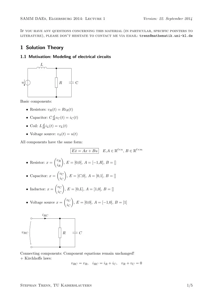
1.1 Motivation: Modeling of electrical circuits

u L R C Basic components:

• Resistors: vR(t) = RiR(t)
• Capacitor: C d

dtvC(t) = iC(t)

• Coil: L d

dtiL(t) = vL(t)

• Voltage source: vS(t) = u(t)

All components have the same form: E ˙ x = Ax + Bu E,A ∈ Rℓ×n, B ∈ Rℓ×m

• Resistor: x =

vR iR

• , E = [0,0], A = [−1,R], B = []
• Capacitor: x =

vC iC

• , E = [C,0], A = [0,1], B = []
• Inductor: x =

vC iC

• , E = [0,L], A = [1,0], B = []
• Voltage source x =

vC iC

• , E = [0,0], A = [−1,0], B = [1]

iRC R C vRC Connecting components: Component equations remain unchanged! + Kirchhoffs laws: vRC = vR, iRC = iR + iC, vR + vC = 0 Stephan Trenn, TU Kaiserslautern 1/5

SAMM DAEs, Elgersburg 2014: Lecture 1 Version: 22. September 2014 Results again in E ˙ x = Ax + Bu with x = (vR, iR, vC, iC, vRC, iRC) and E =       C       , A =       −1 R 1 1 −1 −1 −1 1 1 1       Altogether: x = (vR, iR, vC, iC, vL, iL, vS, iS) E =             C L             , A =             −1 R 1 1 1 1 1 −1 −1 1 −1 1 1 1 1             , B =             1            

1.2 DAEs: What is different to ODEs

Example:   1   ˙ x =   1 1   x +   f1 f2 f3   ˙ x2 = x1 + f1 x1 = −f1 − ˙ f2 0 = x2 + f2 x2 = −f2 0 = f3 no restriction on x3 Observations:

• For fixed inhomogeneity, initial values cannot be chosen arbitrarily (x1(0) = −f1(0) − ˙

f2(0), x2(0) = f2(0))

• For fixed inhomogeneity, solution not uniquely determined by initial value (x3 free)
• Inhomogeneity not arbitrary
• structural restrictions (f3 = 0)
• differentiability restrictions ( ˙

f2 must be well defined)

1.3 Special DAE-cases

a) ODEs: ˙ x = Ax + f

• Initial values: arbitrary
• Solution uniquely determined by f and x(0)
• Inhomogeneity constraints
• no structural constraints
• no differentiability constraints

Stephan Trenn, TU Kaiserslautern 2/5

SAMM DAEs, Elgersburg 2014: Lecture 1 Version: 22. September 2014 b) nilpotent DAEs:       1 ... ... ... 1       ˙ x = x + f ⇔ 0 = x1 + f1 − → x1 = −f1 ˙ x1 = x2 + f2 − → x2 = −f2 − ˙ f1 . . . . . . . . . ˙ xn−1 = xn + fn − → xn = −

n

• i=1

f(n−i)

i

In general: N ˙ x = x + f with N nilpotent, i.e. Nn = 0

N d dt

⇒ N2¨ x = N ˙ x + N ˙ f = x + f + N ˙ f

N d dt

⇒ · · ·

N d dt

⇒ 0 = Nnx(n) = x +

n−1

• i=0

Nif(i) ⇒ x = −

n−1

• i=0

Nif(i) is unique solution of N ˙ x = x + f

• Initial values: fixed by inhomogeneity
• Solution uniquely determined by f
• Inhomogeneity constraints:
• no structural constraints
• differentiability constraints: (Nif)(i) needs to be well defined

c) underdetermined DAEs

n − 1 n

   1 ... ... 1    ˙ x =    1 ... ... 1    x + f ⇔    ˙ x1 . . . ˙ xn−1    =       1 ... ... ... 1          x1 . . . xn−1    +      . . . xn      + f ⇔ ODE with additional “input” xn

• Initial values: arbitrary
• Solution not uniquely determined by x(0) and f
• Inhomogeneity constraints: none

Stephan Trenn, TU Kaiserslautern 3/5

SAMM DAEs, Elgersburg 2014: Lecture 1 Version: 22. September 2014 d) overdetermined DAEs

n + 1 n

         1 ... ... ... ... 1          ˙ x =          1 ... ... ... ... 1          x + f ⇔       1 ... ... ... 1      

• N

˙ x = x +    f1 . . . fn    ∧ ˙ xn = fn+1 ⇔ x = −

n−1

• i=0

Nif(i) ∧ ˙ xn = −

n

• i=1

fn−i+1

i !

= fn+1

• ⇔

n+1

• i=1

f(n+1−i)

i

= 0

• Initial valus: fixed by inhomogeneity
• Solution uniquely determined by f
• Inhomogeneity constraints
• structural constraint: n+1

i=1 f(n+1−i) i

= 0

• differentiability constraint: fn+1−i

i

needs to be well defined We will see: There are no other cases!

1.4 Solution behavior, equivalence and normal forms

Solution behavior of E ˙ x = Ax + f B[E,A,I] :=

• (x,f)
• x ∈ C1(R → Rn), f : R → Rm, E ˙

x = Ax + f

• Fact 1: For any invertible matrix S ∈ Rm×m:

(x,f) ∈ B[E,A,I] ⇔ (x,Sf) ∈ B[SE,SA,I] Fact 2: For coordinate transformation x = Tz, T ∈ Rn×n invertible: (x,f) ∈ B[E,A,I] ⇔ (T −1x,f) ∈ B[ET,AT,I] Together: (x,f) ∈ B[E,A,I] ⇔ (T −1,Sf) ∈ B[SET,SAT,I] Definition 1. (E1,A1), (E2,A2) are called equivalent :⇔ (E2,A2) = (SE1T, SA1T) short: (E1,A1) ∼ = (E2,A2)

• r

(E1,A1)

S,T

∼ = (E2,A2) Stephan Trenn, TU Kaiserslautern 4/5

SAMM DAEs, Elgersburg 2014: Lecture 1 Version: 22. September 2014 Theorem 1 (Quasi-Kronecker Form). For any E,A ∈ Rℓ×m, ∃ invertible S ∈ Rℓ×ℓ and invertible T ∈ Rn×n: (E,A)

S,T

∼ =                     EU I N EO           ,           AU J I AO                     where (EU,AU) consists of underdetermined blocks on the diagonal, N is nilpotent, and (EO,AO) consists of overdetermined diagonal bolcks Example:     1   ,   1 1     ∼ =     1 |   ,   1 1 |     Corollary 1. E ˙ x = Ax+f has solution x for any sufficiently smooth f and each solution x is uniquely determined by x(0) and f ⇔ (E,A) ∼ = I N

• ,

J I

• , N nilpotent

(E,A) is then called regular. Stephan Trenn, TU Kaiserslautern 5/5