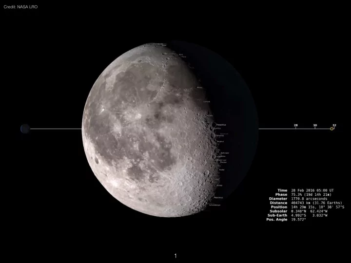
1 Nakajima & Stevenson (2014) arXiv:1401.3036 Constraints: - - PowerPoint PPT Presentation

1
SMART_READER_LITE
LIVE PREVIEW

1 Nakajima & Stevenson (2014) arXiv:1401.3036 Constraints: - - PowerPoint PPT Presentation

Credit: NASA LRO 1 Nakajima & Stevenson (2014) arXiv:1401.3036 Constraints: Orbital Configuration Magma Ocean/ Lack of Volatiles Isotopes 2 Benz et al. (1987) Canup et al. (2013) Nakajima & Stevenson (2014) Icarus 71, 30


slide-1
SLIDE 1

1

Credit: NASA LRO

slide-2
SLIDE 2

Constraints:

  • Orbital Configuration
  • Magma Ocean/

Lack of Volatiles

  • Isotopes

2

Nakajima & Stevenson (2014) arXiv:1401.3036

slide-3
SLIDE 3

3

Benz et al. (1987) Icarus 71, 30 Canup et al. (2013) Icarus 222, 1 Nakajima & Stevenson (2014) arXiv:1401.3036 Hosono et al. (2016) arXiv:1602.00843 Reinhardt & Stadel (2017) arXiv:1701.08296 Kegerreis et al. (2019) arXiv:1901.09934

slide-4
SLIDE 4

4

…But what about magnetic fields?

Gammie et al. (2016) arXiv:1607.02132

slide-5
SLIDE 5

Proto- Earth

A B

5

slide-6
SLIDE 6

Proto- Earth

A B

5

slide-7
SLIDE 7

Proto- Earth

A B

5

slide-8
SLIDE 8

Proto- Earth

A B

5

slide-9
SLIDE 9

6

A First-Take At A Magnetized Giant Impact?

Configuration:

  • Gamma Law EOS
  • Adiabatic, Ideal MHD
  • FFT Gravity Solver (Periodic BC’s)
  • Cartesian, Uniform Grid

python configure.py —-prob=giant_impact -b —-grav=fft -fft (—-nghost=4 -mpi -hdf5)

slide-10
SLIDE 10

7

  • ()

/

  • / ⊕

ρ/ρ

Setup: Planets

Visualization with

slide-11
SLIDE 11

8

  • / ⊕

/ ⊕

~ B = r ⇥ ( ~ Aφ · b(r))

b(r) = ( A exp ⇣ −

ψ r2

cutoff−r2

⌘ for r < rcutoff

  • therwise

~ Aφ = ⇡I0$2r2 c(r2

0 + r2)3/2

✓ 1 + 15r2

0(r2 0 + $2)

8(r2

0 + r2)2

Setup: Setup Dipole Magnetic Fields

c.f., Ruiz & Shapiro (2017) arXiv:1709.00414

slide-12
SLIDE 12

9

Athena++ 10243 Giant Impact Simulation (Linear Resolution ~ 200 km) 643 meshblocks Magnetized, 1 kG at poles Cartesian, HLLD, FFT Self-Gravity, PPM, Periodic BCs

Visualization with

slide-13
SLIDE 13

10

Visualization with

slide-14
SLIDE 14

11

Balbus & Hawley 1992

δ

  • ×
  • ×
  • ×
  • ×
  • ×

× ×

  • δ
  • ×
  • ×
  • ×

× ×

  • δϕ
  • ×
  • ×
  • ×
  • ×

× × ×

  • δ
  • ×
  • ×
  • ×
  • ×

× ×

  • δ
  • ×
  • ×
  • ×

× ×

  • δϕ
  • ×
  • ×
  • ×
  • 2 R⊕

3 R⊕

slide-15
SLIDE 15

12

Visualization with

slide-16
SLIDE 16

13

Conclusions:

  • First numerical simulations of magnetized, Moon-forming giant impacts

(Mullen & Gammie 2019, in prep).

  • Onset of the MRI in a Moon-forming giant impact debris disk with growth

times in agreement with linear theory (Balbus & Hawley 1992).

  • Magnetic turbulence promotes mixing (Gammie et al. 2016, arXiv:

1607.02132).

  • Accretion leads to processing through the boundary layer producing high

entropy material; the boundary layer sources sound waves (c.f., Belyaev et

  • al. 2016: arXiv:1709.01197) that propagate throughout the disk.

Caveats:

  • Quantitative studies of mixing from magnetic turbulence requires composition

variables (in development).

  • Need to separately track iron cores and silicate mantles (in development,

see Dr. Roseanne Cheng’s talk this afternoon!).

  • Need better treatment of EOS (in development).
  • Need open-BCs for gravitational potential (in development).
  • Not all of the protolunar disk will be well-coupled to the magnetic field; need

fast and efficient algorithms for resistive MHD (in development).

slide-17
SLIDE 17

14

Future Directions:

Multi-Material Evolution:

…towards multi-material resistive MHD with realistic EOS for astrophysical/planetary science applications

Realistic (Tabular) EOS: Resistive MHD with Super-Time-Stepping:

python configure.py —-prob=mm_triple_pt (-b) —mm —-nmat=3 python configure.py —-prob=shock_tube —-eos=general/eos_table python configure.py —-prob=resistive_diffusion —sts

slide-18
SLIDE 18

Thank You! Questions?

15

  • P. D. Mullen

UIUC Email: pmullen2@illinois.edu GitHub: pdmullen