1 Global Value Numbering (cont) Role of SSA Form Idea [Alpern, - PowerPoint PPT Presentation

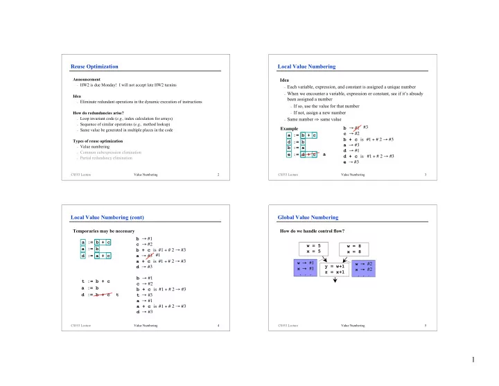
Reuse Optimization Local Value Numbering Announcement Idea − HW2 is due Monday! I will not accept late HW2 turnins − Each variable, expression, and constant is assigned a unique number − When we encounter a variable, expression or constant, see if it’s already Idea been assigned a number − Eliminate redundant operations in the dynamic execution of instructions − If so, use the value for that number − If not, assign a new number How do redundancies arise? − Loop invariant code ( e.g., index calculation for arrays) − Same number ⇒ same value − Sequence of similar operations ( e.g., method lookup) #3 Example b → #1 − Same value be generated in multiple places in the code c → #2 a := b + c b + c is #1 + # 2 → #3 Types of reuse optimization d := b a → # 3 − Value numbering b := a d → #1 − Common subexpression elimination a e := d + c d + c is #1 + # 2 → #3 − Partial redundancy elimination e → #3 CS553 Lecture Value Numbering 2 CS553 Lecture Value Numbering 3 Local Value Numbering (cont) Global Value Numbering Temporaries may be necessary How do we handle control flow? b → #1 a := b + c c → #2 w = 5 w = 8 a := b b + c is #1 + # 2 → #3 x = 5 x = 8 #1 d := a + c a → # 3 a + c is #1 + # 2 → #3 w → #1 w → #2 y = w+1 d → #3 x → #1 x → #2 z = x+1 . . . . . . b → #1 t := b + c c → #2 a := b b + c is #1 + # 2 → #3 d := b + c t t → # 3 a → # 1 a + c is #1 + # 2 → #3 d → #3 CS553 Lecture Value Numbering 4 CS553 Lecture Value Numbering 5 1

Global Value Numbering (cont) Role of SSA Form Idea [Alpern, Wegman, and Zadeck 1988] SSA form is helpful − Partition program variables into congruence classes − Allows us to avoid data-flow analysis − All variables in a particular congruence class have the same value − Variables correspond to values − SSA form is helpful a = b a 1 = b . . . . . . a = c a 2 = c a not congruent to Congruence classes: Approaches to computing congruence classes . . . . . . { a 1 , b }, { a 2 , c }, { a 3 , d } anything − Pessimistic a = d a 3 = d − Assume no variables are congruent (start with n classes) − Iteratively coalesce classes that are determined to be congruent − Optimistic − Assume all variables are congruent (start with one class) − Iteratively partition variables that contradict assumption − Slower but better results CS553 Lecture Value Numbering 6 CS553 Lecture Value Numbering 7 Basis Pessimistic Global Value Numbering Idea Idea − If x and y are congruent then f(x) and f(y) are congruent − Initially each variable is in its own congruence class − Consider each assignment statement s (reverse postorder in CFG) ta = a tb = b − Update LHS value number with hash of RHS x and y are x = f(a,b) congruent − Identical value number ⇒ congruence y = f(ta,tb) − Use this fact to combine (pessimistic) or split (optimistic) classes Why reverse postorder? Problem − Ensures that when we consider an assignment statement, we have already considered definitions that reach the RHS operands − This is not true for φ -functions a 1 & b 1 congruent? a a 1 = x 1 a 2 = y 1 b 1 = x 1 b 2 = y 1 a 2 & b 2 congruent? b n m Postorder: d, c, e, b, f, a a 3 = φ (a 1 ,a 2 ) b 3 = φ (b 1 ,b 2 ) c e f n m a 3 & b 3 congruent? Solution: Label φ -functions with join point d CS553 Lecture Value Numbering 8 CS553 Lecture Value Numbering 9 2

Algorithm Snag! for each assignment of the form: “ x = f(a,b) ” Problem ValNum[x] ← UniqueValue() // same for a and b − Our algorithm assumes that we consider operands before variables that depend upon it for each assignment of the form: “ x = f(a,b) ” (in reverse postorder) − Can’t deal with code containing loops! ValNum[x] ← Hash(f ⊕ ValNum[a] ⊕ ValNum[b]) #1 i 1 = 1 a 1 Solution #2 b 1 − Ignore back edges i 1 #3 w 1 = b 1 w 2 = a 1 w 1 #4 #2 − Make conservative (worst case) assumption for previously unseen x 1 = b 1 x 2 = a 1 x 1 #5 #2 variable ( i.e., assume its in it’s own congruence class) w 2 #6 #1 x 2 #7 #1 w 3 = φ n (w 1 , w 2 ) φ n (#2,#1) → #12 w 3 #8 x 3 = φ n (x 1 , x 2 ) φ n (#2,#1) → #12 x 3 #9 y 1 = w 3 +i 1 +(#12,#3) → #13 y 1 #10 z 1 = x 3 +i 1 +(#12,#3) → #13 z 1 #11 CS553 Lecture Value Numbering 10 CS553 Lecture Value Numbering 11 Optimistic Global Value Numbering Splitting Idea Initially − Initially all variables in one congruence class − Variables computed using the same function are placed in the same class − Split congruence classes when evidence of non-congruence arises P P’ x 1 = f(a 1 ,b 1 ) − Variables that are computed using different functions . . . x 1 y 1 z 1 − Variables that are computed using functions with non-congruent y 1 = f(c 1 ,d 1 ) operands . . . z 1 = f(e 1 ,f 1 ) Iteratively Q − Split classes when corresponding a 1 c 1 operands are in different classes − Example: a 1 and c 1 are congruent, but e 1 is congruent to neither CS553 Lecture Value Numbering 12 CS553 Lecture Value Numbering 13 3

Splitting (cont) Algorithm worklist ← ∅ Definitions for each function f − Suppose P and Q are sets representing congruence classes C f ← ∅ − Q splits P for each i into two sets for each assignment of the form “x = f(a,b)” − P \ i Q contains variables in P whose i th operand is in Q C f ← C f ∪ { x } − P / i Q contains variables in P whose i th operand is not in Q worklist ← worklist ∪ {C f } CC ← CC ∪ {C f } − Q properly splits P if neither resulting set is empty while worklist ≠ ∅ Delete some D from worklist P Q for each class C properly split by D (at operand i) x 1 = f(a 1 ,b 1 ) CC ← CC – C . . . x 1 y 1 z 1 a 1 c 1 worklist ← worklist – C y 1 = f(c 1 ,d 1 ) Create new congruence classes C j ← {C \ i D} and C k ← {C / i D} . . . CC ← CC ∪ C j ∪ C k z 1 = f(e 1 ,f 1 ) P \ 1 Q P / 1 Q worklist ← worklist ∪ C j ∪ C k Note: see paper for optimization CS553 Lecture Value Numbering 14 CS553 Lecture Value Numbering 15 Example Comparing Optimistic and Pessimistic Differences SSA code Congruence classes − Handling of loops S 0 { x 0 } x 0 = 1 − Pessimistic makes worst-case assumptions on back edges S 1 { y 0 } y 0 = 2 S 2 { x 1 , y 1 , z 1 } − Optimistic requires actual contradiction to split classes x 1 = x 0 +1 S 3 { x 1 ,z 1 } y 1 = y 0 +1 S 4 { y 1 } z 1 = x 0 +1 w 0 = 5 x 0 = 5 Worklist: S 0 ={ x 0 }, S 1 ={ y 0 }, S 2 ={ x 1 , y 1 ,z 1 } , S 3 ={ x 1 ,z 1 }, S 4 ={ y 1 } S 0 psplit S 0 ? no S 0 psplit S 1 ? no S 0 psplit S 2 ? yes! w 1 = φ (w 0 ,w 2 ) x 1 = φ (x 0 ,x 2 ) S 2 \ 1 S 0 = { x 1 , z 1 } = S 3 w 2 = w 1 +1 x 2 = x 1 +1 S 2 / 1 S 0 = { y 1 } = S 4 CS553 Lecture Value Numbering 16 CS553 Lecture Value Numbering 17 4

Role of SSA Next Time Single global result Lecture − Single def reaches each use − Midterm Review − No data (flow value) at each point − Send questions you would like answered at the Midterm Review No data flow analysis − Optimistic: Iterate over congruence classes, not CFG nodes − Pessimistic: Visit each assignment once φ -functions − Make data-flow merging explicit − Treat like normal functions CS553 Lecture Value Numbering 18 CS553 Lecture Value Numbering 19 5