1 2 CS 532: 3D Computer Vision Lecture 2 Enrique Dunn - - PowerPoint PPT Presentation

1

CS 532: 3D Computer Vision Lecture 2

Enrique Dunn edunn@stevens.edu Lieb 310

2

Image Formation

Based on slides by John Oliensis

3

Lecture Outline

• Single View Geometry
• 2D projective transformations

– Homographies

• Robust estimation

– RANSAC

• Radial distortion
• Two-view geometry

Based on slides by R. Hartley, A. Zisserman,

• M. Pollefeys and S. Seitz

4

Image Formation

Pinhole camera

image plane (film) pinhole Object Virtual image light ray

5

Projection Equation

• 2D world è 1D image

camera center “Film”

f

(focal length)

Object

x z

Image

6

( )

, , X Y Z

ˆ X ˆ Y ˆ Z Y x y f X Z

x X y f Y Z = =

( ) ( )

, , f Y x X Z y =

Projection Equation: 3D

Similar triangles:

7

Perspective Projection: Properties

• 3D points è image points
• 3D straight lines è image straight lines
• 3D Polygons è image polygons

8

Polyhedra Project to Polygons

(since lines project to lines)

9

Properties: Distant objects are smaller

B’ C’

10

Sin Single le Vie View Geome metry ry

Rich ichard rd Hart rtle ley y and An Andre rew Zisse isserma rman Ma Marc rc Po Polle llefeys ys

Modified by Philippos Mordohai

11

Homogeneous Coordinates

• 3-D points represented as 4-D vectors (X Y Z 1)T
• Equality defined up to scale

– (X Y Z 1)T ~ (WX WY WZ W)T

• Useful for perspective projection à makes equations

linear C m M1 M2

12

Pinhole camera model

T T

Z fY Z fX Z Y X ) / , / ( ) , , (

• ⎟

⎟ ⎟ ⎟ ⎟ ⎠ ⎞ ⎜ ⎜ ⎜ ⎜ ⎜ ⎝ ⎛ ⎥ ⎥ ⎥ ⎦ ⎤ ⎢ ⎢ ⎢ ⎣ ⎡ = ⎟ ⎟ ⎟ ⎠ ⎞ ⎜ ⎜ ⎜ ⎝ ⎛ ⎟ ⎟ ⎟ ⎟ ⎟ ⎠ ⎞ ⎜ ⎜ ⎜ ⎜ ⎜ ⎝ ⎛ 1 1 1 Z Y X f f Z fY fX Z Y X

• linear projection in homogeneous coordinates!

13

The Pinhole Camera

Z fY y Z fX x = =

14

Principal Point Offset

T y x T

p Z fY p Z fX Z Y X ) / , / ( ) , , ( + +

• principal point

T y x p

p ) , (

⎟ ⎟ ⎟ ⎟ ⎟ ⎠ ⎞ ⎜ ⎜ ⎜ ⎜ ⎜ ⎝ ⎛ ⎥ ⎥ ⎥ ⎦ ⎤ ⎢ ⎢ ⎢ ⎣ ⎡ = ⎟ ⎟ ⎟ ⎠ ⎞ ⎜ ⎜ ⎜ ⎝ ⎛ + + ⎟ ⎟ ⎟ ⎟ ⎟ ⎠ ⎞ ⎜ ⎜ ⎜ ⎜ ⎜ ⎝ ⎛ 1 1 1 Z Y X p f p f Z Zp fY Zp fX Z Y X

y x y x

• 15

⎟ ⎟ ⎟ ⎟ ⎟ ⎠ ⎞ ⎜ ⎜ ⎜ ⎜ ⎜ ⎝ ⎛ ⎥ ⎥ ⎥ ⎦ ⎤ ⎢ ⎢ ⎢ ⎣ ⎡ = ⎟ ⎟ ⎟ ⎠ ⎞ ⎜ ⎜ ⎜ ⎝ ⎛ + + 1 1 Z Y X p f p f Z Zp fY Zp fX

y x x x

[ ]

cam

X | I K x =

⎥ ⎥ ⎥ ⎦ ⎤ ⎢ ⎢ ⎢ ⎣ ⎡ = 1

y x

p f p f K

calibration matrix

Principal Point Offset

16

Hands On: Image Formation

• For a 640 by 480 image with focal length

equal to 640 pixels, find 3D points that are marginally visible at the four borders of the image

• Increase and decrease the focal length.

What happens?

17

Camera Rotation and Translation

( )

C ~

• X

~ R X ~

cam =

X 1 C ~ R R 1 1 C ~ R R Xcam ⎥ ⎦ ⎤ ⎢ ⎣ ⎡ − = ⎟ ⎟ ⎟ ⎟ ⎟ ⎠ ⎞ ⎜ ⎜ ⎜ ⎜ ⎜ ⎝ ⎛ ⎥ ⎦ ⎤ ⎢ ⎣ ⎡ − = Z Y X

18

X 1 C ~ R R 1 1 C ~ R R Xcam ⎥ ⎦ ⎤ ⎢ ⎣ ⎡ − = ⎟ ⎟ ⎟ ⎟ ⎟ ⎠ ⎞ ⎜ ⎜ ⎜ ⎜ ⎜ ⎝ ⎛ ⎥ ⎦ ⎤ ⎢ ⎣ ⎡ − = Z Y X

[ ]

cam

X | I K x =

[ ]X

C ~ | I KR x − =

[ ]

t | R K P = C ~ R t − =

PX x =

19

Camera Rotation and Translation

Intrinsic Parameters

• Camera deviates from pinhole

s: skew fx ≠ fy: different magnification in x and y (cx cy): optical axis does not pierce image plane exactly at the center

• Usually:

rectangular pixels: square pixels: principal point known:

⎥ ⎥ ⎥ ⎦ ⎤ ⎢ ⎢ ⎢ ⎣ ⎡ = 1 ) cos(

• v

f u s f af K

⎥ ⎥ ⎥ ⎦ ⎤ ⎢ ⎢ ⎢ ⎣ ⎡ = 1

y y x x

c f c s f K

( )

⎟ ⎠ ⎞ ⎜ ⎝ ⎛ = 2 , 2 , h w c c

y x

y x

f f s = = 0

• r

⎥ ⎥ ⎥ ⎦ ⎤ ⎢ ⎢ ⎢ ⎣ ⎡ = 1 γ y f x sf f K

20

Extrinsic Parameters

⎥ ⎥ ⎦ ⎤ ⎢ ⎢ ⎣ ⎡ = ⎥ ⎦ ⎤ ⎢ ⎣ ⎡ = 1 t) (R

• R

M' 1 t R M

(1x3) 3x1 T (3x3) T (1x3) (3x1) (3x3)

Scene motion Camera motion

21

Projection matrix

• Includes coordinate transformation and

camera intrinsic parameters

⎥ ⎥ ⎥ ⎥ ⎦ ⎤ ⎢ ⎢ ⎢ ⎢ ⎣ ⎡ ⎥ ⎥ ⎥ ⎦ ⎤ ⎢ ⎢ ⎢ ⎣ ⎡ = ⎥ ⎥ ⎥ ⎦ ⎤ ⎢ ⎢ ⎢ ⎣ ⎡ λ 1 1

34 33 32 31 24 23 22 21 14 13 12 11

Z Y X p p p p p p p p p p p p y x

22

• Everything we need to know about a pinhole

camera

• Unambiguous
• Can be decomposed into parameters

Projection matrix

• Mapping from 2-D to 3-D is a function of

internal and external parameters

[ ]

⎥ ⎥ ⎥ ⎥ ⎦ ⎤ ⎢ ⎢ ⎢ ⎢ ⎣ ⎡ − ⎥ ⎥ ⎥ ⎦ ⎤ ⎢ ⎢ ⎢ ⎣ ⎡ = ⎥ ⎥ ⎥ ⎦ ⎤ ⎢ ⎢ ⎢ ⎣ ⎡ 1 | 1 1 λ Z Y X t R R c f c s f y x

y y x x T T

[ ]X

t R R K x

T T −

= | λ

PX x = λ

23

Hands On: Camera Motion

• Choose a few 3D points visible to a camera

at the origin. (f=500, w=500, h=500)

• Now, move the camera by 2 units of length
• n the z axis. What happens to the images of

the points?

• Rotate the points by 45 degrees about the z

axis of the camera and then translate them by 5 units on the z axis away from the camera. What are the new images of the points?

24

Projective Transformations in 2D

A projectivity is an invertible mapping h from P2 to itself such that three points x1,x2,x3 lie on the same line if and

• nly if h(x1),h(x2),h(x3) do.

Definition: A mapping h:P2→P2 is a projectivity if and only if there exist a non-singular 3x3 matrix H such that for any point in P2 reprented by a vector x it is true that h(x)=Hx Theorem: Definition: Projective transformation

⎟ ⎟ ⎟ ⎠ ⎞ ⎜ ⎜ ⎜ ⎝ ⎛ ⎥ ⎥ ⎥ ⎦ ⎤ ⎢ ⎢ ⎢ ⎣ ⎡ = ⎟ ⎟ ⎟ ⎠ ⎞ ⎜ ⎜ ⎜ ⎝ ⎛

3 2 1 33 32 31 23 22 21 13 12 11 3 2 1

' ' ' x x x h h h h h h h h h x x x x x' H =

• r

8DOF

projectivity=collineation=projective transformation=homography

25

Mapping between planes

central projection may be expressed by x’=Hx

(application of theorem)

26

Removing Projective Distortion

33 32 31 13 12 11 3 1

' ' ' h y h x h h y h x h x x x + + + + = =

33 32 31 23 22 21 3 2

' ' ' h y h x h h y h x h x x y + + + + = =

( )

13 12 11 33 32 31

' h y h x h h y h x h x + + = + +

( )

23 22 21 33 32 31

' h y h x h h y h x h y + + = + +

select four points in a plane with known coordinates (linear in hij) (2 constraints/point, 8DOF ⇒ 4 points needed) Remarks: no calibration at all necessary, better ways to compute (see later)

27

A Hierarchy of Transformations

Projective linear group Affine group (last row (0,0,1)) Euclidean group (upper left 2x2 orthogonal) Oriented Euclidean group (upper left 2x2 det 1) Alternatively, characterize transformation in terms of elements

• r quantities that are preserved or invariant

e.g. Euclidean transformations leave distances unchanged

28

Class I: Isometries

(iso=same, metric=measure)

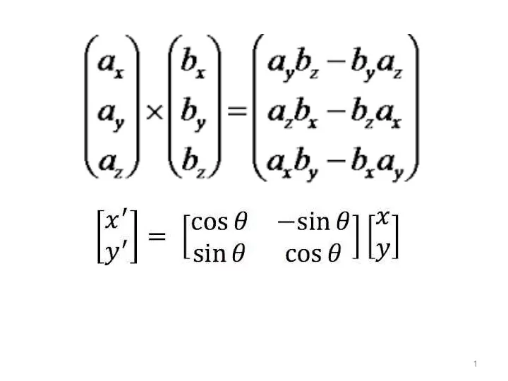
⎟ ⎟ ⎟ ⎠ ⎞ ⎜ ⎜ ⎜ ⎝ ⎛ ⎥ ⎥ ⎥ ⎦ ⎤ ⎢ ⎢ ⎢ ⎣ ⎡ − = ⎟ ⎟ ⎟ ⎠ ⎞ ⎜ ⎜ ⎜ ⎝ ⎛ 1 1 cos sin sin cos 1 ' ' y x t t y x

y x

θ θ ε θ θ ε 1 ± = ε 1 = ε 1 − = ε

• rientation preserving:
• rientation reversing:

x x x' ⎥ ⎦ ⎤ ⎢ ⎣ ⎡ = = 1 t

T

R HE

I R R =

T

special cases: pure rotation, pure translation 3DOF (1 rotation, 2 translation) Invariants: length, angle, area

29

Class II: Similarities

(isometry + scale)

⎟ ⎟ ⎟ ⎠ ⎞ ⎜ ⎜ ⎜ ⎝ ⎛ ⎥ ⎥ ⎥ ⎦ ⎤ ⎢ ⎢ ⎢ ⎣ ⎡ − = ⎟ ⎟ ⎟ ⎠ ⎞ ⎜ ⎜ ⎜ ⎝ ⎛ 1 1 cos sin sin cos 1 ' ' y x t s s t s s y x

y x

θ θ θ θ x x x' ⎥ ⎦ ⎤ ⎢ ⎣ ⎡ = = 1 t

T

R H s

S

I R R =

T

also know as equi-form (shape preserving) metric structure = structure up to similarity (in literature) 4DOF (1 scale, 1 rotation, 2 translation) Invariants: ratios of length, angle, ratios of areas, parallel lines

30

Class III: Affine Transformations

⎟ ⎟ ⎟ ⎠ ⎞ ⎜ ⎜ ⎜ ⎝ ⎛ ⎥ ⎥ ⎥ ⎦ ⎤ ⎢ ⎢ ⎢ ⎣ ⎡ = ⎟ ⎟ ⎟ ⎠ ⎞ ⎜ ⎜ ⎜ ⎝ ⎛ 1 1 1 ' '

22 21 12 11

y x t a a t a a y x

y x

x x x' ⎥ ⎦ ⎤ ⎢ ⎣ ⎡ = = 1 t

T

A H A

non-isotropic scaling! (2DOF: scale ratio and orientation) 6DOF (2 scale, 2 rotation, 2 translation) Invariants: parallel lines, ratios of parallel lengths, ratios of areas

( ) ( ) ( )

φ φ θ DR R R A − =

⎥ ⎦ ⎤ ⎢ ⎣ ⎡ =

2 1

λ λ D

31

Class VI: Projective Transformations

x v x x' ⎥ ⎦ ⎤ ⎢ ⎣ ⎡ = = v

P T

t A H

Action is non-homogeneous over the plane 8DOF (2 scale, 2 rotation, 2 translation, 2 line at infinity) Invariants: cross-ratio of four points on a line (ratio of ratios)

( )

T 2 1,

v v v =

32

Overview of Transformations

⎥ ⎥ ⎥ ⎦ ⎤ ⎢ ⎢ ⎢ ⎣ ⎡ 1

22 21 12 11 y x

t a a t a a ⎥ ⎥ ⎥ ⎦ ⎤ ⎢ ⎢ ⎢ ⎣ ⎡ 1

22 21 12 11 y x

t sr sr t sr sr ⎥ ⎥ ⎥ ⎦ ⎤ ⎢ ⎢ ⎢ ⎣ ⎡

33 32 31 23 22 21 13 12 11

h h h h h h h h h ⎥ ⎥ ⎥ ⎦ ⎤ ⎢ ⎢ ⎢ ⎣ ⎡ 1

22 21 12 11 y x

t r r t r r

Projective 8dof Affine 6dof Similarity 4dof Euclidean 3dof

Concurrency, collinearity,

• rder of contact (intersection,

tangency, inflection, etc.), cross ratio Parallellism, ratio of areas, ratio of lengths on parallel lines (e.g midpoints), linear combinations of vectors (centroids). The line at infinity l∞ Ratios of lengths, angles. The circular points I,J lengths, areas.

33

Homework 1

Warp the basketball court from this image to a new image so that it appears as if the new image was taken from directly above What are we missing?

34

Image Warping

Slides by Steve Seitz

35

Image Transformations

36

Parametric (Global) Warping

• Transformation T is a coordinate-changing machine:

p’ = T(p)

• What does it mean that T is global?

– It is the same for any point p – It can be described by just a few numbers (parameters)

• T is represented as a matrix (see prev. slides):

p’ = M*p

37

Image Warping

Given a coordinate transform (x’,y’) = h(x,y) and a source image f(x,y), how do we compute a transformed image g(x’,y’) = f(T(x,y))?

38

Forward Warping

Send each pixel f(x,y) to its corresponding location (x’,y’) = T(x,y) in the second image Q: what if the pixel lands “between” two pixels?

39

Forward Warping

Send each pixel f(x,y) to its corresponding location (x’,y’) = T(x,y) in the second image Q: what if the pixel lands “between” two pixels? A: Distribute color among neighboring pixels (splatting)

40

Inverse Warping

• Get each pixel g(x’,y’) from its corresponding

location (x,y) = T-1(x’,y’) in the first image

• Q: what if pixel comes from “between” two

pixels?

41

Inverse Warping

• Get each pixel g(x’,y’) from its corresponding location

(x,y) = T-1(x’,y’) in the first image

• Q: what if pixel comes from “between” two pixels?
• A: interpolate color value from neighbors

– Bilinear interpolation typically used

42

Bilinear Interpolation

43

Forward vs. Inverse Warping

• Which is better?
• ...

44

Parameter Estimation

Slides by R. Hartley, A. Zisserman and M. Pollefeys

45

Homography: Number of Measurements Required

• At least as many independent equations as

degrees of freedom required

• Example:

Hx x'=

⎥ ⎥ ⎥ ⎦ ⎤ ⎢ ⎢ ⎢ ⎣ ⎡ ⎥ ⎥ ⎥ ⎦ ⎤ ⎢ ⎢ ⎢ ⎣ ⎡ = ⎥ ⎥ ⎥ ⎦ ⎤ ⎢ ⎢ ⎢ ⎣ ⎡ ʹ″ ʹ″ 1 1 λ

33 32 31 23 22 21 13 12 11

y x h h h h h h h h h y x

2 independent equations / point 8 degrees of freedom 4x2≥8

46

Approximate solutions

• Minimal solution

4 points yield an exact solution for H

• More points

– No exact solution, because measurements are inexact (“noise”) – Search for “best” according to some cost function – Algebraic or geometric/statistical cost

47

Direct Linear Transformation (DLT)

i i

Hx x = ʹ″ Hx x = × ʹ″

i i

⎟ ⎟ ⎟ ⎟ ⎠ ⎞ ⎜ ⎜ ⎜ ⎜ ⎝ ⎛ =

i i i i

x h x h x h Hx

3 2 1 T T T

⎟ ⎟ ⎟ ⎟ ⎠ ⎞ ⎜ ⎜ ⎜ ⎜ ⎝ ⎛ ʹ″ − ʹ″ ʹ″ − ʹ″ ʹ″ − ʹ″ = × ʹ″

i i i i i i i i i i i i i i

y x x w w y x h x h x h x h x h x h Hx x

1 2 3 1 2 3 T T T T T T

h h h x x x x x x

3 2 1

= ⎟ ⎟ ⎟ ⎠ ⎞ ⎜ ⎜ ⎜ ⎝ ⎛ ⎥ ⎥ ⎥ ⎦ ⎤ ⎢ ⎢ ⎢ ⎣ ⎡ ʹ″ ʹ″ − ʹ″ − ʹ″ ʹ″ ʹ″ −

T T T T T T T T T i i i i i i i i i i i i

x y x w y w

( )

T i i i i

w y x ʹ″ ʹ″ ʹ″ = ʹ″ , , x

h A =

i

48

Direct Linear Transformation (DLT)

Equations are linear in h

h h h x x x x x x

3 2 1

= ⎟ ⎟ ⎟ ⎠ ⎞ ⎜ ⎜ ⎜ ⎝ ⎛ ⎥ ⎥ ⎥ ⎦ ⎤ ⎢ ⎢ ⎢ ⎣ ⎡ ʹ″ ʹ″ − ʹ″ − ʹ″ ʹ″ ʹ″ −

T T T T T T T T T i i i i i i i i i i i i

x y x w y w

A A A

3 2 1

= ʹ″ + ʹ″ + ʹ″

i i i i i i

w y x

h A =

i

Only 2 of 3 are linearly independent (indeed, 2 eq/pt)

49

Direct Linear Transformation (DLT)

h h h x x x x

3 2 1

= ⎟ ⎟ ⎟ ⎠ ⎞ ⎜ ⎜ ⎜ ⎝ ⎛ ⎥ ⎦ ⎤ ⎢ ⎣ ⎡ ʹ″ − ʹ″ ʹ″ ʹ″ −

T T T T T T i i i i i i i i

x w y w

(only drop third row if wi’≠0)

• Holds for any homogeneous

representation, e.g. (xi’,yi’,1)

50

Direct Linear Transformation (DLT)

• Solving for H

Ah = h A A A A

4 3 2 1

= ⎥ ⎥ ⎥ ⎥ ⎦ ⎤ ⎢ ⎢ ⎢ ⎢ ⎣ ⎡

Size of A is 8x9, but rank 8 Trivial solution is h=09

T is not interesting

1-D null-space yields solution of interest, pick for example the one with

1 h =

51

Direct Linear Transformation (DLT)

• Over-determined solution

No exact solution because of inexact measurement i.e. “noise”

h A A A

n 2 1

= ⎥ ⎥ ⎥ ⎥ ⎦ ⎤ ⎢ ⎢ ⎢ ⎢ ⎣ ⎡

• Find approximate solution
• Additional constraint needed to avoid 0, e.g.
• not possible, so minimize

1 h = Ah

Ah =

52

DLT Algorithm

Objective Given n≥4 2D to 2D point correspondences {xi↔xi’}, determine the 2D homography matrix H such that xi’=Hxi Algorithm (i) For each correspondence xi ↔xi’ compute Ai. Usually

• nly two first rows needed.

(ii) Assemble n 2x9 matrices Ai into a single 2nx9 matrix A (iii) Obtain SVD of A. Solution for h is last column of V (iv) Determine H from h

53

Inhomogeneous solution

⎟ ⎟ ⎠ ⎞ ⎜ ⎜ ⎝ ⎛− = ⎥ ⎦ ⎤ ⎢ ⎣ ⎡ − − − − − ' ' h ~ ' ' ' ' ' ' ' ' ' '

i i i i i i i i i i i i i i i i i i i i i i i i

x w y w x y x x w w w y w x y y y x w w w y w x

Since h can only be computed up to scale, pick hj=1, e.g. h9=1, and solve for 8-vector h

~

Solve using Gaussian elimination (4 points) or using linear least-squares (more than 4 points) However, if h9=0 this approach fails Also poor results if h9 close to zero Therefore, not recommended

54

Normalizing Transformations

• Since DLT is not invariant to transformations,

what is a good choice of coordinates?

e.g. – Translate centroid to origin – Scale to a average distance to the origin – Independently on both images

2

1 norm

1 2 / 2 / T

−

⎥ ⎥ ⎥ ⎦ ⎤ ⎢ ⎢ ⎢ ⎣ ⎡ + + = h h w w h w

55

Importance of Normalization

h h h 1 1

3 2 1

= ⎟ ⎟ ⎟ ⎠ ⎞ ⎜ ⎜ ⎜ ⎝ ⎛ ⎥ ⎦ ⎤ ⎢ ⎣ ⎡ ʹ″ − ʹ″ − ʹ″ − ʹ″ ʹ″ ʹ″ − ʹ″ − ʹ″ −

i i i i i i i i i i i i i i

x y x x x y x y y y x y y x

~102 ~102 ~102 ~102 ~104 ~104 ~102 1 1

• rders of magnitude difference!

Monte Carlo simulation for identity computation based on 5 points (not normalized ↔ normalized)

56

Normalized DLT Algorithm

Objective Given n≥4 2D to 2D point correspondences {xi↔xi’}, determine the 2D homography matrix H such that xi’=Hxi Algorithm (i) Normalize points (ii) Apply DLT algorithm to (iii) Denormalize solution

, x ~ x ~

i i

ʹ″ ↔

i norm i i norm i

x T x ~ , x T x ~ ʹ″ ʹ″ = ʹ″ =

norm

• 1

norm T

H ~ T H ʹ″ =

57

RANSAC

Slides by R. Hartley, A. Zisserman and M. Pollefeys

58

Robust Estimation

• What if set of matches contains gross outliers?

59

RANSAC

Objective Robust fit of model to data set S which contains outliers Algorithm (i) Randomly select a sample of s data points from S and instantiate the model from this subset. (ii) Determine the set of data points Si which are within a distance threshold t of the model. The set Si is the consensus set of samples and defines the inliers of S. (iii) If the subset of Si is greater than some threshold T, re- estimate the model using all the points in Si and terminate (iv) If the size of Si is less than T, select a new subset and repeat the above. (v) After N trials the largest consensus set Si is selected, and the model is re-estimated using all the points in the subset Si

60

How Many Samples?

Choose N so that, with probability p, at least one random sample is free from outliers. e.g. p=0.99

( ) ( )

( )

s

e p N − − − = 1 1 log / 1 log

( )

( )

p e

N s

− = − − 1 1 1

proportion of outliers e

s 5% 10% 20% 25% 30% 40% 50% 2 2 3 5 6 7 11 17 3 3 4 7 9 11 19 35 4 3 5 9 13 17 34 72 5 4 6 12 17 26 57 146 6 4 7 16 24 37 97 293 7 4 8 20 33 54 163 588 8 5 9 26 44 78 272 1177

61

Acceptable Consensus Set

• Typically, terminate when inlier ratio reaches expected

ratio of inliers

( )n

e T − = 1

62

Adaptively Determining the Number of Samples

e is often unknown a priori, so pick worst case, e.g. 50%,

and adapt if more inliers are found, e.g. 80% would yield

e=0.2

– N=∞, sample_count =0 – While N >sample_count repeat

• Choose a sample and count the number of inliers
• Set e=1-(number of inliers)/(total number of points)
• Recompute N from e
• Increment the sample_count by 1

– Terminate

( ) ( )

( ) ( )

s

e p N − − − = 1 1 log / 1 log

63

Other robust algorithms

• RANSAC maximizes number of inliers
• LMedS minimizes median error
• Not recommended: case deletion, iterative

least-squares, etc.

64

Automatic Computation of H

Objective Compute homography between two images Algorithm (i) Interest points: Compute interest points in each image (ii) Putative correspondences: Compute a set of interest point matches based on some similarity measure (iii) RANSAC robust estimation: Repeat for N samples (a) Select 4 correspondences and compute H (b) Calculate the distance d⊥ for each putative match (c) Compute the number of inliers consistent with H (d⊥<t) Choose H with most inliers (iv) Optimal estimation: re-estimate H from all inliers by minimizing ML cost function with Levenberg-Marquardt (v) Guided matching: Determine more matches using prediction by computed H Optionally iterate last two steps until convergence

65

Determine Putative Correspondences

• Compare interest points

Similarity measure: – SAD, SSD, ZNCC in small neighborhood

• If motion is limited, only consider interest points with

similar coordinates

66

Example: robust computation

Interest points (500/image) (640x480) Putative correspondences (268) (Best match,SSD<20,±320) Outliers (117) (t=1.25 pixel; 43 iterations) Inliers (151) Final inliers (262)

#in

1-e adapt. N 6 2% 20M 10 3% 2.5M 44 16% 6,922 58 21% 2,291 73 26% 911 151 56% 43

67

Radial Distortion and Undistortion

Slides by R. Hartley, A. Zisserman and M. Pollefeys

68

short and long focal length

Radial Distortion

69

70

71

Correction of distortion Choice of the distortion function and center

Computing the parameters of the distortion function (i) Minimize with additional unknowns (ii) Straighten lines (iii) …

72

Typical Undistortion Model

73

Why Undistort?

Two-View Geometry

Slides by R. Hartley, A. Zisserman and M. Pollefeys

74

(i) Correspondence geometry: Given an image point x in the first image, how does this constrain the position of the corresponding point x’ in the second image? (ii) Camera geometry (motion): Given a set of corresponding image points {xi ↔x’i}, i=1,…,n, what are the cameras P and P’ for the two views? (iii) Scene geometry (structure): Given corresponding image points xi ↔x’i and cameras P, P’, what is the position of (their pre- image) X in space?

Three questions:

75

C, C’, x, x’ and X are coplanar

The Epipolar Geometry

76

What if only C,C’,x are known?

The Epipolar Geometry

77

All points on π project on l and l’

78

The Epipolar Geometry

Family of planes π and lines l and l’ Intersection in e and e’

79

The Epipolar Geometry

epipoles e, e’ = intersection of baseline with image plane = projection of projection center in other image = vanishing point of camera motion direction an epipolar plane = plane containing baseline (1-D family) an epipolar line = intersection of epipolar plane with image (always come in corresponding pairs)

80

The Epipolar Geometry

Example: Converging Cameras

81

(simple for stereo → rectification)

Exa Examp mple le: Mo Motio ion Pa Para ralle llel l to Ima mage Pla Plane

82

e e’

Example: Forward Motion

83

The Fundamental Matrix F

algebraic representation of epipolar geometry

l' x

we will see that mapping is a (singular) correlation (i.e. projective mapping from points to lines) represented by the fundamental matrix F

84

correspondence condition

Fx x'T =

The fundamental matrix satisfies the condition that for any pair of corresponding points x↔x’ in the two images

( )

l' x'T =

85

The Fundamental Matrix F

( )

λC x P λ X + =

+

( )

I PP =

+

[ ]

+ ×

= P P' e' F x P P' C P' l

+

× =

(note: doesn’t work for C=C’ ⇒ F=0)

x P+ ( )

λ X

86

The Fundamental Matrix F

F is the unique 3x3 rank 2 matrix that satisfies x’TFx=0 for all x↔x’

(i) Transpose: if F is fundamental matrix for (P,P’), then FT is fundamental matrix for (P’,P) (ii) Epipolar lines: l’=Fx & l=FTx’ (iii) Epipoles: on all epipolar lines, thus e’TFx=0, ∀x ⇒e’TF=0, similarly Fe=0 (iv) F has 7 d.o.f. , i.e. 3x3-1(homogeneous)-1(rank2) (v) F is a correlation, projective mapping from a point x to a line l’=Fx (not a proper correlation, i.e. not invertible)

87

The Fundamental Matrix F

Two View Geometry Computation: Linear Algorithm

Fx x'T =

separate known from unknown

' ' ' ' ' '

33 32 31 23 22 21 13 12 11

= + + + + + + + + f yf xf f y yf y xf y f x yf x xf x

[ ][ ]

, , , , , , , , 1 , , , ' , ' , ' , ' , ' , '

T 33 32 31 23 22 21 13 12 11

= f f f f f f f f f y x y y y x y x y x x x

(data) (unknowns) (linear)

Af = f 1 ' ' ' ' ' ' 1 ' ' ' ' ' '

1 1 1 1 1 1 1 1 1 1 1 1

= ⎥ ⎥ ⎦ ⎤ ⎢ ⎢ ⎣ ⎡

n n n n n n n n n n n n

y x y y y x y x y x x x y x y y y x y x y x x x

• For every match (m,m´):

88

Benefits from having F

• Given a pixel in one image, the

corresponding pixel has to lie on epipolar line

• Search space reduced from 2-D to 1-D

89

simplify stereo matching by warping the images Apply projective transformation so that epipolar lines correspond to horizontal scanlines e e map epipole e to (1,0,0) try to minimize image distortion problem when epipole in (or close to) the image

He 1 = ⎥ ⎥ ⎦ ⎤ ⎢ ⎢ ⎣ ⎡

Image Pair Rectification

90

Pla Planar r Rect ctif ifica icatio ion

Bring two views to standard stereo setup (moves epipole to ∞) (not possible when in/close to image) (standard approach)

91

92