1 The Cost of Feature Transformation Feature Rescaling } Not every - - PowerPoint PPT Presentation

1
SMART_READER_LITE
LIVE PREVIEW

1 The Cost of Feature Transformation Feature Rescaling } Not every - - PowerPoint PPT Presentation

Feature Engineering } As we saw with polynomial regression, we often want to transform our data in order to get better results from a machine learning algorithm } We often get better results by: Changing how features are represented. 1. Adding


slide-1
SLIDE 1

1

Class #10: Feature Engineering

Machine Learning (COMP 135): M. Allen, 20 Feb. 20

1

Feature Engineering

} As we saw with polynomial regression, we often want to

transform our data in order to get better results from a machine learning algorithm

} We often get better results by:

1.

Changing how features are represented.

2.

Adding new features.

3.

Deleting/ignoring some features.

Thursday, 20 Feb. 2020 Machine Learning (COMP 135) 2

2

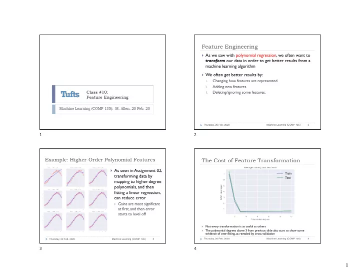
Example: Higher-Order Polynomial Features

} As seen in Assignment 02,

transforming data by mapping to higher-degree polynomials, and then fitting a linear regression, can reduce error

} Gains are most significant

at first, and then error starts to level off

Thursday, 20 Feb. 2020 Machine Learning (COMP 135) 3

3

The Cost of Feature Transformation

}

Not every transformation is as useful as others

}

The polynomial degrees above 3 from previous slide also start to show some evidence of over-fitting, as revealed by cross-validation

Thursday, 20 Feb. 2020 Machine Learning (COMP 135) 4

4

slide-2
SLIDE 2

2 The Cost of Feature Transformation

} Not every transformation

is useful—at very high polynomials, some of the mathematics of the linear regression libraries in sklearn break down

} Mathematically, we expect

better and better fits

} In practice, the method

ceases working effectively, and models are generally useless

Thursday, 20 Feb. 2020 Machine Learning (COMP 135) 5

5

Feature Rescaling Input: Each numeric feature has arbitrary min/max

} Some in [0, 1], Some in [-5, 5], Some [-3333, -2222]

Transformed feature vector

} Set each feature value f to have [0, 1] range

} min_f = minimum observed in training set } max_f = maximum observed in training set

6 Machine Learning (COMP 135)

φ(xn)f = xnf − minf maxf − minf

Thursday, 20 Feb. 2020

6 Input: Each feature is numeric, has arbitrary scale Transformed feature vector

  • Set each feature value f to have zero mean, unit variance

Empirical mean observed in training set Empirical standard deviation observed in training set

Feature Standardization

φ(xn)f = xnf − µf σf

7 Machine Learning (COMP 135)

µf σf

Thursday, 20 Feb. 2020

7

Feature Standardization

} Treats each feature as “Normal(0, 1)” } Typical range will be -3 to +3

} If original data is approximately normal

} Also called z-score transform

8 Machine Learning (COMP 135)

φ(xn)f = xnf − µf σf

Thursday, 20 Feb. 2020

8

slide-3
SLIDE 3

3 Best Subset Selection

} Main issue: too many subsets

} There are O(2p) such collections of features } For problems with large feature-sets, this grows quickly infeasible

9 Machine Learning (COMP 135) Thursday, 20 Feb. 2020

9

Forward Stepwise Selection

1.

Start with zero feature model (guess mean)

} Store as M_0

  • 2. Add best scoring single feature (among all F)

} Store as M_1

  • 3. For each size k = 2, … F

} Try each possible not-included feature (F – k + 1) } Add best scoring feature to the model M_k-1 } Store as M_k

  • 4. Pick best among M_0, M_1, … M_F,

based upon the validation data

10 Machine Learning (COMP 135) Thursday, 20 Feb. 2020

10

Best vs Forward Stepwise

11 Machine Learning (COMP 135)

Easy to find cases where forward stepwise ‘s greedy approach doesn’t deliver best possible subset.

Thursday, 20 Feb. 2020

11

Backwards Stepwise Selection

The basic forward model can also be run backwards:

1.

Start with all features

2.

Gradually test all models with one feature removed from each

3.

Repeat to remove 2, 3, … features, down to single- feature versions

12 Machine Learning (COMP 135) Thursday, 20 Feb. 2020

12

slide-4
SLIDE 4

4 Next Week

} Special schedule: Class Wednesday & Thursday } T

  • pics: Clustering methods

} Readings linked from class schedule page } Assignments: } Homework 03: due Wednesday, 26 Feb., 9:00 AM

} Logistic regression & decision trees

} Project 01: due Monday, 09 March, 5:00 PM

} Feature engineering and classification for image data

} Midterm Exam: Wednesday, 11 March } Office Hours: 237 Halligan } Monday, 10:30 AM – Noon } T

uesday, 9:00 AM – 1:00 PM

} TA hours can be found on class website

Thursday, 20 Feb. 2020 Machine Learning (COMP 135) 13

13