We are familiar with the Fourier Series in which a function x of - - PowerPoint PPT Presentation

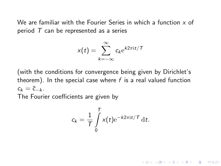
We are familiar with the Fourier Series in which a function x of period T can be represented as a series x(t) =

∞

• k=−∞

ckek2πit/T (with the conditions for convergence being given by Dirichlet’s theorem). In the special case where f is a real valued function ck = ¯ c−k. The Fourier coefficients are given by ck = 1 T

T

• x(t)e−k2πit/T dt.

CN ( the vectors uk = 1

N

• e2πki(n−1)/NN

n=1 form an orthonormal

basis with respect to the standard inner product. We can therefore regard a sequence of N samples of a function f , x = (x(t0 + (n − 1)δ))N

n=1 as a vector (here δ is the sampling

interval) and define the Discrete Fourier Transform DFT of x as ˆ x = (x · un)N

n=1 ∈ CN

(1) Then we have x =

N

• k=1

ˆ xkuk. (2)

The Fourier Transform is defined by ˆ x(s) =

∞

• −∞

x(t)e−2πistdt and can be inverted using the Inverse Fourier Transform x(t) = 1 2π

∞

• −∞

ˆ x(s)e2πistdt.

A cos(2πft + φ) is said to have amplitude A, frequency f and phase φ More generally consider cos θ(t), where typically θ(t) = 2πf0t + φ(t). We define the instantaneous frequency as finst(t) = θ′(t) 2π = f + φ′(t) 2π With this interpretation, if you have a signal m(t) and you want to frequency modulate a sinusoidal signal with frequency f0, the modulated signal is xFM(t) = cos 2π  f0t +

t

• m(t) dt

 

The Hilbert Transform of a real function x(t) is defined by Hx(t) = P.V. ∞

−∞

x(s) t − s ds, also

• Hx(s) = −i sign(s)ˆ

x(s) which makes a numerical approximation easier to calculate If x(t) is a real valued signal the complex signal z(t) = x(t) + iHx(t) is a complex analytic function restricted to the real axis. If z(t) = exp iθ(t) instantaneous phase is then θ(t) = arg z(t)