1 Expectimax Pseudocode Expectimax Example 10 1/2 1/6 1/3 5 8 - - PDF document

1

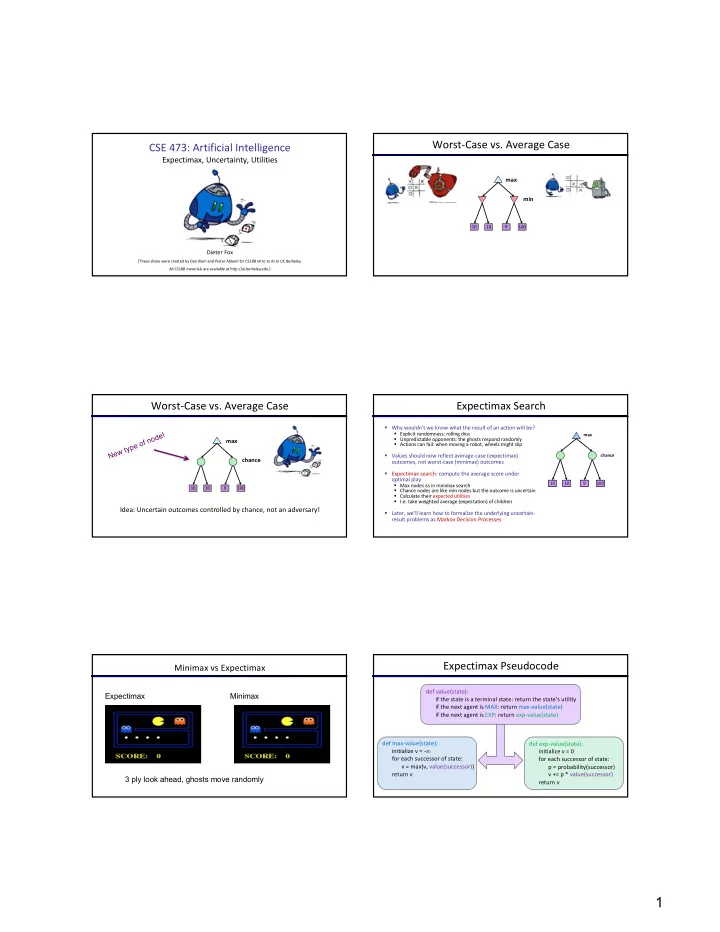
CSE 473: Artificial Intelligence

Expectimax, Uncertainty, Utilities

Dieter Fox

Worst-Case vs. Average Case

max min

Worst-Case vs. Average Case

max chance

Idea: Uncertain outcomes controlled by chance, not an adversary!

Expectimax Search

§ Why wouldn’t we know what the result of an action will be? § Explicit randomness: rolling dice § Unpredictable opponents: the ghosts respond randomly § Actions can fail: when moving a robot, wheels might slip § Values should now reflect average-case (expectimax)

• utcomes, not worst-case (minimax) outcomes

§ Expectimax search: compute the average score under

• ptimal play

§ Max nodes as in minimax search § Chance nodes are like min nodes but the outcome is uncertain § Calculate their expected utilities § I.e. take weighted average (expectation) of children § Later, we’ll learn how to formalize the underlying uncertain- result problems as Markov Decision Processes

Minimax vs Expectimax

Expectimax Minimax 3 ply look ahead, ghosts move randomly

Expectimax Pseudocode

def value(state): if the state is a terminal state: return the state’s utility if the next agent is MAX: return max-value(state) if the next agent is EXP: return exp-value(state) def exp-value(state): initialize v = 0 for each successor of state: p = probability(successor) v += p * value(successor) return v def max-value(state): initialize v = -∞ for each successor of state: v = max(v, value(successor)) return v

2

Expectimax Pseudocode

def exp-value(state): initialize v = 0 for each successor of state: p = probability(successor) v += p * value(successor) return v 5 7 8 24

• 12

1/2 1/3 1/6

v = (1/2) (8) + (1/3) (24) + (1/6) (-12) = 10 10

Expectimax Example

Expectimax Pruning?

• 12

10

Depth-Limited Expectimax

Probabilities Reminder: Probabilities

§ A random variable represents an event whose outcome is unknown § A probability distribution is an assignment of weights to outcomes § Example: Traffic on freeway

§ Some laws of probability (more later):

§ As we get more evidence, probabilities may change:

0.25 0.50 0.25

3

§ The expected value of a function of a random variable is the average, weighted by the probability distribution over

• utcomes

§ Example: How long to get to the airport?

Reminder: Expectations

0.25 0.50 0.25 Probability: 20 min 30 min 60 min Time:

35 min

+ +

§ In expectimax search, we have a probabilistic model

• f how the opponent (or environment) will behave in

any state

§ Model could be a simple uniform distribution (roll a die) § Model could be sophisticated and require a great deal of computation § We have a chance node for any outcome out of our control:

• pponent or environment

§ The model might say that adversarial actions are likely!

§ For now, assume each chance node magically comes along with probabilities that specify the distribution

• ver its outcomes

What Probabilities to Use? Informed Probabilities

§ Let’s say you know that your opponent is sometimes lazy. 20% of the time, she moves randomly, but usually (80%) she runs a depth 2 minimax to decide her move § Question: What tree search should you use?

§ Answer: Expectimax!

§ To figure out EACH chance node’s probabilities, you have to run a simulation of your opponent § This kind of thing gets very slow very quickly § Even worse if you have to simulate your

• pponent simulating you…

§ … except for minimax, which has the nice property that it all collapses into one game tree

Modeling Assumptions The Dangers of Optimism and Pessimism

Dangerous Optimism

Dangerous Pessimism

Video of Demo World Assumptions Random Ghost – Expectimax Pacman

4

Video of Demo World Assumptions Adversarial Ghost – Minimax Pacman Video of Demo World Assumptions Adversarial Ghost – Expectimax Pacman Video of Demo World Assumptions Random Ghost – Minimax Pacman

Assumptions vs. Reality

Adversarial Ghost Random Ghost Minimax Pacman Won 5/5

• Avg. Score: 483

Won 5/5

• Avg. Score: 493

Expectimax Pacman Won 1/5

• Avg. Score: -303

Won 5/5

• Avg. Score: 503

Other Game Types Example: Backgammon

5

Mixed Layer Types

§ E.g. Backgammon § Expectiminimax

§ Environment is an extra “random agent” player that moves after each min/max agent § Each node computes the appropriate combination of its children

Example: Backgammon

§ Dice rolls increase b: 21 possible rolls with 2 dice § Backgammon ~ 20 legal moves § Depth 2 = 20 x (21 x 20)3 = 1.2 x 109 § As depth increases, probability of reaching a given search node shrinks § So usefulness of search is diminished § So limiting depth is less damaging § But pruning is trickier… § Historic AI (1992): TDGammon uses depth-2 search + very good evaluation function + reinforcement learning: world-champion level play § 1st AI world champion in any game!

Different Types of Ghosts?

Stupid Devilish Smart

Multi-Agent Utilities

§ What if the game is not zero-sum, or has multiple players? § Generalization of minimax:

§ Terminals have utility tuples § Node values are also utility tuples § Each player maximizes its own component § Can give rise to cooperation and competition dynamically…

Utilities Maximum Expected Utility

§ Why should we average utilities? § Principle of maximum expected utility:

§ A rational agent should chose the action that maximizes its expected utility, given its knowledge

§ Questions:

§ Where do utilities come from? § How do we know such utilities even exist? § How do we know that averaging even makes sense? § What if our behavior (preferences) can’t be described by utilities?

6

What Utilities to Use?

§ For worst-case minimax reasoning, terminal function scale doesn’t matter § We just want better states to have higher evaluations (get the ordering right) § We call this insensitivity to monotonic transformations § For average-case expectimax reasoning, we need magnitudes to be meaningful

Utilities

§ Utilities are functions from outcomes (states of the world) to real numbers that describe an agent’s preferences § Where do utilities come from?

§ In a game, may be simple (+1/-1) § Utilities summarize the agent’s goals § Theorem: any “rational” preferences can be summarized as a utility function

§ We hard-wire utilities and let behaviors emerge

§ Why don’t we let agents pick utilities? § Why don’t we prescribe behaviors?

Utilities: Uncertain Outcomes

Getting ice cream Get Single Get Double Oops Whew!

Preferences

§ An agent must have preferences among:

§ Prizes: A, B, etc. § Lotteries: situations with uncertain prizes

§ Notation:

§ Preference: § Indifference:

A B

p 1-p

A Lottery A Prize A

Rationality

§ We want some constraints on preferences before we call them rational, such as: § For example: an agent with intransitive preferences can be induced to give away all of its money

§ If B > C, then an agent with C would pay (say) 1 cent to get B § If A > B, then an agent with B would pay (say) 1 cent to get A § If C > A, then an agent with A would pay (say) 1 cent to get C

Rational Preferences

) ( ) ( ) ( C A C B B A ! ! ! Þ Ù Axiom of Transitivity:

7

Rational Preferences

Theorem: Rational preferences imply behavior describable as maximization of expected utility

The Axioms of Rationality

§ Theorem [Ramsey, 1931; von Neumann & Morgenstern, 1944]

§ Given any preferences satisfying these constraints, there exists a real-valued function U such that: § I.e. values assigned by U preserve preferences of both prizes and lotteries!

§ Maximum expected utility (MEU) principle:

§ Choose the action that maximizes expected utility § Note: an agent can be entirely rational (consistent with MEU) without ever representing or manipulating utilities and probabilities § E.g., a lookup table for perfect tic-tac-toe, a reflex vacuum cleaner

MEU Principle Human Utilities Utility Scales

§ Normalized utilities: u+ = 1.0, u- = 0.0 § Micromorts: one-millionth chance of death, useful for paying to reduce product risks, etc. § QALYs: quality-adjusted life years, useful for medical decisions involving substantial risk § Note: behavior is invariant under positive linear transformation § With deterministic prizes only (no lottery choices), only

• rdinal utility can be determined, i.e., total order on prizes

§ Utilities map states to real numbers. Which numbers? § Standard approach to assessment (elicitation) of human utilities: § Compare a prize A to a standard lottery Lp between

§ “best possible prize” u+ with probability p § “worst possible catastrophe” u- with probability 1-p § Adjust lottery probability p until indifference: A ~ Lp § Resulting p is a utility in [0,1]

Human Utilities

0.999999 0.000001

No change Pay $30 Instant death

Money

§ Money does not behave as a utility function, but we can talk about the utility of having money (or being in debt) § Given a lottery L = [p, $X; (1-p), $Y] § The expected monetary value EMV(L) is p*X + (1-p)*Y § U(L) = p*U($X) + (1-p)*U($Y) § Typically, U(L) < U( EMV(L) ) § In this sense, people are risk-averse § When deep in debt, people are risk-prone

8

Example: Insurance

§ Consider the lottery [0.5, $1000; 0.5, $0]

§ What is its expected monetary value? ($500) § What is its certainty equivalent?

§ Difference of $100 is the insurance premium

§ It’s win-win: you’d rather have the $400 and the insurance company would rather have the lottery (their utility curve is flat and they have many lotteries)

Example: Human Rationality?

§ Famous example of Allais (1953)

§ A: [0.8, $4k; 0.2, $0] § B: [1.0, $3k; 0.0, $0] § C: [0.2, $4k; 0.8, $0] § D: [0.25, $3k; 0.75, $0]

§ Most people prefer B > A, C > D § But if U($0) = 0, then

§ B > A è U($3k) > 0.8 U($4k) § C > D è0.8 U($4k) > U($3k)

Kahneman & Tversky

Choose between

Option A § 33% $2500 § 66% $2400 § 01% Option B § 100% $2400

[18] [82]*

Kahneman & Tversky

Choose between

Option C § 33% $2500 § 67% Option D § 34% $2400 § 66%

[83]* [17]

Kahneman & Tversky

Choose between

Option A § 33% $2500 § 66% $2400 § 01% Option B § 100% $2400

[18] [82]*

Option C § 33% $2500 § 67% Option D § 34% $2400 § 66%

[83]* [17]

• 66% chance of $2400 from both options

Recommended