[PDF] - 1 Q- -digest digest Q Example Example Exact data: frequency PDF Document

SLIDE 1

1

10/25/05 Jie Gao, CSE590-fall05 1

Robust Aggregation in Sensor Robust Aggregation in Sensor Networks Networks

Jie Gao

Computer Science Department Stony Brook University

10/25/05 Jie Gao, CSE590-fall05 2

Papers Papers

[Shrivastava04] Nisheeth Shrivastava, Chiranjeeb

Buragohain, Divy Agrawal, Subhash Suri, Medians and Beyond: New Aggregation Techniques for Sensor Networks, ACM SenSys '04, Nov. 3-5, Baltimore, MD.

[Nath04] Suman Nath, Phillip B. Gibbons, Zachary Anderson,

and Srinivasan Seshan, Synopsis Diffusion for Robust Aggregation in Sensor Networks". In proceedings of ACM SenSys'04.

[Considine04] Jeffrey Considine, Feifei Li, George Kollios,

and John Byers, Approximate Aggregation Techniques for Sensor Databases, Proc. ICDE, 2004.

[Przydatek03] Bartosz Przydatek, Dawn Song, Adrian Perrig,

SIA: Secure Information Aggregation in Sensor Networks, Sensys’03.

10/25/05 Jie Gao, CSE590-fall05 3

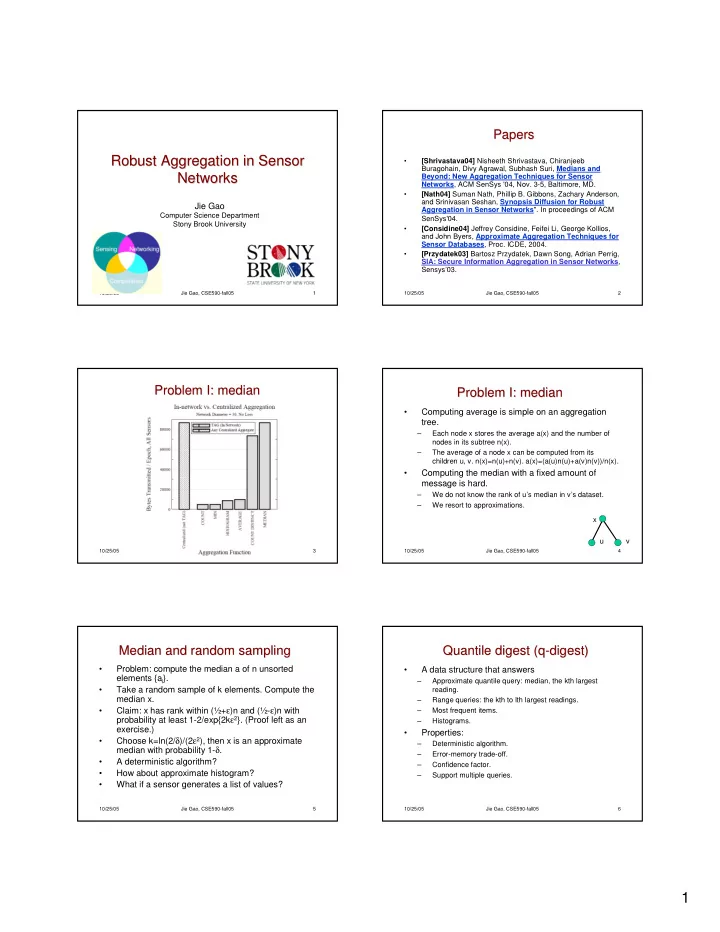
Problem I: median Problem I: median

10/25/05 Jie Gao, CSE590-fall05 4

Problem I: median Problem I: median

Computing average is simple on an aggregation

tree.

– Each node x stores the average a(x) and the number of nodes in its subtree n(x). – The average of a node x can be computed from its children u, v. n(x)=n(u)+n(v). a(x)=(a(u)n(u)+a(v)n(v))/n(x).

Computing the median with a fixed amount of

message is hard.

– We do not know the rank of u’s median in v’s dataset. – We resort to approximations. x u v

10/25/05 Jie Gao, CSE590-fall05 5

Median and random sampling Median and random sampling

Problem: compute the median a of n unsorted

elements {ai}.

Take a random sample of k elements. Compute the

median x.

Claim: x has rank within (½+ε)n and (½-ε)n with

probability at least 1-2/exp{2kε2}. (Proof left as an exercise.)

Choose k=ln(2/δ)/(2ε2), then x is an approximate

median with probability 1-δ.

A deterministic algorithm?
How about approximate histogram?
What if a sensor generates a list of values?

10/25/05 Jie Gao, CSE590-fall05 6

Quantile Quantile digest (q digest (q-

digest)

digest)

A data structure that answers

– Approximate quantile query: median, the kth largest reading. – Range queries: the kth to lth largest readings. – Most frequent items. – Histograms.

Properties:

– Deterministic algorithm. – Error-memory trade-off. – Confidence factor. – Support multiple queries.

SLIDE 2

2

10/25/05 Jie Gao, CSE590-fall05 7

Q Q-

digest

digest

Exact data: frequency of data value {f1, f2,…,fσ}.
Compress the data:

– detailed information concerning frequent data are preserved; – less frequently occurring values are lumped into larger buckets resulting in information loss.

Buckets: the nodes in a binary partition of the range

[1, σ]. Each bucket v has range [v.min, v.max].

Only store non-zero buckets.
Digest property:

– Count(v) n/k. (except leaf) – Count(v) + Count(p) + Count(s) > n/k. (except root)

parent sibling

10/25/05 Jie Gao, CSE590-fall05 8

Example Example

Input data bucketed Q-digest

Information loss

10/25/05 Jie Gao, CSE590-fall05 9

Construct a q Construct a q-

digest

digest

Each sensor

constructs a q- digest based

n its value.
Check the

digest property bottom up: two “small” children’s count are added up and moved to the parent.

10/25/05 Jie Gao, CSE590-fall05 10

Merging two q Merging two q-

digests

digests

Merge q-digests

from two children

Add up the

values in buckets

Re-evaluate the

digest property bottom up.

Information loss: t undercounts since some of its value appears on ancestors.

10/25/05 Jie Gao, CSE590-fall05 11

Space complexity and error bound Space complexity and error bound

1. A q-digest with compression parameter k has at most 3k buckets.

By property 2, for buckets Q,

– v∈Q [Count(v) + Count(p) + Count(s)] > |Q| n/k. – v∈Q [Count(v) + Count(p) + Count(s)] 3v∈QCount(v)=3n. – |Q|<3k.

Any value that should be counted in v can be

present in one of the ancestors. 1. Count(v) has max error logσ⋅n/k.

– Error(v) ancestor p Count(p) ancestor p n/k logσ⋅n/k.

2. MERGE maintains the same relative error.

– Error(v) i Error(vi) i logσ⋅ni/k logσ⋅n/k.

10/25/05 Jie Gao, CSE590-fall05 12

Median and Median and quantile quantile query query

Given q∈(0, 1), find the value

whose rank is qn.

Relative error ε=|r-qn|/n, where r is

the true rank.

Post-order traversal on Q, sum the

counts of all nodes visited before a node v, which is the lower bound

n the # of values less than v.max.

Report it when it is first time larger than qn.

Error bound: logσ /k = 3logσ /m,

where m=3k is the storage bound for each sensor.

SLIDE 3

3

10/25/05 Jie Gao, CSE590-fall05 13

Other queries Other queries

Inverse quantile: given a value, determine its rank.

– Traverse the tree in post-order, report the sum of counts v for which x>v.max, which is within [rank(x), rank(x)+εn]

Range query: find # values in range [l,h].

– Perform two inverse quantile queries and take the

difference. Error bound is 2εn.
Frequent items: given s∈(0, 1), find all values

reported by more than sn sensors.

– Count the leaf buckets whose counts are more than sn. – Small false positive: values with count between (s-ε)n and sn may also be reported as frequent.

10/25/05 Jie Gao, CSE590-fall05 14

Simulation setup Simulation setup

A typical aggregation tree (BFS tree) on 40 nodes

in a 200 by 200 area. In the simulation they use 4000~8000 nodes.

10/25/05 Jie Gao, CSE590-fall05 15

Simulation setup Simulation setup

Random data;
Correlated data:3D elevation value from Death

Valley.

10/25/05 Jie Gao, CSE590-fall05 16

Histogram v.s. q Histogram v.s. q-

digest

digest

Comparison of histogram and q-digest.

10/25/05 Jie Gao, CSE590-fall05 17

Tradeoff between error and Tradeoff between error and msg msg size size

10/25/05 Jie Gao, CSE590-fall05 18

Saving on message size Saving on message size

SLIDE 4

4

10/25/05 Jie Gao, CSE590-fall05 19

Problem II: Aggregation along a Problem II: Aggregation along a spanning tree in practice spanning tree in practice

The impact of link dynamics on aggregation tree.
If a link fails, the data from the entire subtree is lost.

– Wrong aggregated value; – Inconsistency.

10/25/05 Jie Gao, CSE590-fall05 20

Problem II: Aggregation along a Problem II: Aggregation along a spanning tree in practice spanning tree in practice

Solution: use multi-path

routing (e.g., DAG) to improve robustness under link dynamics.

But if both paths succeed,

the the same data is received twice!

This is ok for some

aggregation such as MAX, MIN.

How about Count, SUM?

1 2 3 4 5 6

10/25/05 Jie Gao, CSE590-fall05 21

Aggregation along a spanning tree Aggregation along a spanning tree

Problem with spanning tree: Link dynamics
If a link fails, the data from the entire subtree is lost.
Decouple routing and data aggregation.
Use multi-path routing to improve the routing

robustness.

If multiple paths succeed, the sink receives multiple

copies of the same data.

Design an aggregation algorithm that is insensitive

to order and duplications.

10/25/05 Jie Gao, CSE590-fall05 22

Order and duplicate insensitive Order and duplicate insensitive (ODI) synopses (ODI) synopses

Aggregated value is insensitive to the sequence or

duplication of input data.

Small-sizes digests such that any particular sensor

reading is accounted for only once.

– MAX, MIN admit natural ODI synopsis. – ODI synopsis for SUM, COUNT, MEDIAN, AVG are more challenging.

Synopsis generation: SG(⋅).
Synopsis fusion: SF(⋅) takes two synopsis and

generate a new synopsis of the union of input data.

Synopsis evaluation: SE(⋅) translates the synopsis to

the final answer.

10/25/05 Jie Gao, CSE590-fall05 23

ODI synopsis for MAX/MIN ODI synopsis for MAX/MIN

Synopsis generation: SG(⋅).

– Output the value itself.

Synopsis fusion: SF(⋅)

– Take the MAX/MIN of the two input values.

Synopsis evaluation: SE(⋅).

– Output the synopsis.

SG() SF() SE()

10/25/05 Jie Gao, CSE590-fall05 24

ODI correctness ODI correctness

A synopsis diffusion algorithm is ODI-correct if

SF() and SG() are order and duplicate insensitive functions.

Or, if for any aggregation DAG, the resulting

synopsis is identical to the synopsis produced by the canonical left-deep tree.

The final result is independent of the underlying

routing topology.

SLIDE 5

5

10/25/05 Jie Gao, CSE590-fall05 25

ODI ODI-

synopsis

synopsis

Connection to streaming model: data item comes 1 by 1.

10/25/05 Jie Gao, CSE590-fall05 26

Test for ODI correctness Test for ODI correctness

1. SG() preserves duplicates: if two readings are considered duplicates (e.g., two nodes with the same temperature readings), then the same synopsis is generated. 2. SF() is commutative. 3. SF() is associative. 4. SF() is same-synopsis idempotent, SF(s, s)=s. Theorem: The above properties are sufficient and necessary properties for ODI-correctness. Proof idea: transfer an aggregation DAG to a left-deep tree with the same output by using these properties.

10/25/05 Jie Gao, CSE590-fall05 27

Proof of ODI correctness Proof of ODI correctness

1. Start from the DAG. Duplicate a node with out- degree k to k nodes, each with out degree 1. duplicates preserving.

10/25/05 Jie Gao, CSE590-fall05 28

Proof of ODI correctness Proof of ODI correctness

2. Re-order the leaf nodes by the increasing value of the synopsis. Commutative.

10/25/05 Jie Gao, CSE590-fall05 29

Proof of ODI correctness Proof of ODI correctness

3. Re-organize the tree s.t. adjacent leaves with the same value are input to a SF function. Associative.

SF SF SG SF SG r1 SG SG r2 r2 r3

10/25/05 Jie Gao, CSE590-fall05 30

Proof of ODI correctness Proof of ODI correctness

4. Replace SF(s, s) by s. same-synopsis idempotent.

SF SF SG SF SG r1 SG SG r2 r2 r3 SF SF SG SG r1 SG r2 r3

SLIDE 6

6

10/25/05 Jie Gao, CSE590-fall05 31

Proof of ODI correctness Proof of ODI correctness

5. Re-order the leaf nodes by the increasing canonical

rder. Commutative.

10/25/05 Jie Gao, CSE590-fall05 32

Counting distinct elements Counting distinct elements

Each sensor generates a sensor reading. Count the

total number of different readings.

Counting distinct element in a multi-set. (Flajolet

and Martin 1985).

Coin tossing experiments CT(x) = # coin tosses until

the first head occurs or x coin tosses with no heads.

Pr{CT(x)=i} = Pr{i-1 tails and 1 head} =2-i.
Use a pseudo-random generator so that CT(x) is a

hash function. 1

10/25/05 Jie Gao, CSE590-fall05 33

Counting distinct elements Counting distinct elements

Synopsis: a bit vector of

length k>logn.

SG(): output a bit vector s
f length k with CT(k)’s bit

set.

SF(): bit-wise boolean OR
f input s and s’.
SE(): if s is the lowest

index that is still 0, output 2i-1/0.77351. 1 1 OR 1 1 i=3

10/25/05 Jie Gao, CSE590-fall05 34

Counting distinct elements Counting distinct elements

Check the ODI-

correctness:

– Duplication: by the hash

function. The same reading x

generates the same value CT(x). – Boolean OR is commutative, associative, same-synopsis idempotent.

Total storage: O(logn) bits.

1 1 OR 1 1 i=3

10/25/05 Jie Gao, CSE590-fall05 35

Distinct value counter analysis Distinct value counter analysis

Lemma: For i<logn-2loglogn, FM[i]=1 with high

probability (asymptotically close to 1). For i ≥ 3/2logn+δ, with δ ≥ 0, FM[i]=0 with high probability.

The expected value of the first zero is

log(0.7753n)+P(logn)+o(1), where P(u) is a periodic function of u with period 1 and amplitude bounded by 10-5.

The error bound (depending on variance) can be

improved by using multiple copies or stochastic averaging. 1

10/25/05 Jie Gao, CSE590-fall05 36

Sum Sum

Naïve approach: for an item x with value c times,

make c distinct copies (x, j), j=1, …, c. Now use the distinct count algorithm.

When c is large, we set the bits as if we had

performed c successive insertions to the FM sketch.

First set the first δ = logc-loglogc bits to 1.
Those who reached δ follow a binomial distribution:

each item reaches δ with prob 2-δ.

Explicitly insert those that reached bit δ by coin

flipping.

Powerful building block.

SLIDE 7

7

10/25/05 Jie Gao, CSE590-fall05 37

Second moment Second moment

Kth moment µk=Σ xik, xi is the number of

sensor readings with value i.

– µ0 is the number of distinct elements. – µ1 is the sum. – µ2 is the square of L2 norm.

The famous sketch algorithm for frequency

moments can be turned into an ODI easily by using ODI-sum.

The space complexity of approximating the frequency moments, N. Alon, Y. Matias, and M. Szegedy. STOC 1996.

10/25/05 Jie Gao, CSE590-fall05 38

Second moment Second moment

Random hash h(x): {0,1,…,N-1} {-1,1}
Define zi =h(i)
Maintain X = i xizi
E(X2) = E(i xizi)2 = E(i xi

2zi 2)+ E(i,jxixjzizj).

Choose the hash function to be pairwise

independent: Pr{h(i)=a,h(j)=b} = ¼.

E(zi

2)=1, E(zizj)=0.

Now E(X2) = i xi

2.

ODI: Each sensor generates xizi, then use ODI-

sum.

10/25/05 Jie Gao, CSE590-fall05 39

Uniform sample Uniform sample

Each sensor has a reading. Compute a uniform

sample of a given size k.

Synopsis: a sample of k tuples.
SG(): output (value, r, id), where r is a uniform

random number in range [0, 1].

SF(): output the k tuples with the k largest r values.

If there are less than k tuples in total, out them all.

SE(): output the values in s.
ODI-correctness is implied by the “MAX” and union
peration in SF().
Correctness: the largest k random numbers is a

uniform k sample.

10/25/05 Jie Gao, CSE590-fall05 40

Most popular items Most popular items

Return the k values that occur the most frequently

among all the sensor readings

Synopsis: a set of k most popular items.
SG(): output (value, weight) pair, with

weight=CT(k), k>logn.

SF(): for each distinct value v, discard all but the

pair with max weight. Then output the k pairs with max weight.

SE(): output the set of values.
Note: we attach a weight to estimate the frequency.
Many aggregates that can be approximated by

using random samples now have ODI-synopsis, e.g., median

10/25/05 Jie Gao, CSE590-fall05 41

Implicit acknowledgement Implicit acknowledgement

Explicit acknowledgement:

– 3-way handshake. – Used on internet.

Implicit acknowledgement:

– Used on ad hoc wireless networks. – Node u sending to v snoops the subsequent broadcast from v to see if v indeed forwards the message for u. – Explores broadcast property, saves energy.

With aggregation this is problematic.

– Say u sends value x to v, and subsequently hears value z. – U does not know whether or not x is incorporated into z.

u v

10/25/05 Jie Gao, CSE590-fall05 42

Implicit acknowledgement Implicit acknowledgement

ODI-synopsis enables efficient implicit

acknowledgement.

– U sends to v synopsis x. – Afterwards u hears that v transmitting synopsis z. – U verifies whether SF(x, z)=z ?

u v

SLIDE 8

8

10/25/05 Jie Gao, CSE590-fall05 43

Decouple routing with aggregation Decouple routing with aggregation

Use arbitrary multi-path routing schemes to allow

message redundancy to be adaptive to sensor network conditions.

Use Directed Acyclic Graph (DAG) to replace tree.
Rings overlay:

– Query distribution: nodes in ring Rj are j hops from q. – Query aggregation: node in ring Rj wakes up in its allocated time slot and receives message from nodes in Rj+1.

10/25/05 Jie Gao, CSE590-fall05 44

Rings and adaptive rings Rings and adaptive rings

Adaptive rings: cope with network dynamics, node

deletions and insertions, etc.

Each node on ring j monitor the success rate of its

parents on ring j-1.

If the success rate is low, the node connects to
ther node whose transmission is overhead a lot.
Nodes at ring 1 may transmit multiple times to

ensure robustness.

10/25/05 Jie Gao, CSE590-fall05 45

Error of approximate answers Error of approximate answers

Two sources of errors:

– Algorithmic error: due to randomization and approximation. – Communication error: the fraction of sensor readings not accounted for in the final answer.

Algorithmic error depends on the choice of

algorithm and thus relatively controllable.

Communication error depends on the network

dynamics and robustness of routing algorithms.

10/25/05 Jie Gao, CSE590-fall05 46

Simulation results Simulation results

Unaccounted node

10/25/05 Jie Gao, CSE590-fall05 47

Simulation results Simulation results

Relative root mean square error

10/25/05 Jie Gao, CSE590-fall05 48

Conclusion Conclusion

Due to the high dynamics in sensor networks,

robust aggregates that are insensitive to order and duplication are very attractive – they provide the flexibility of using any multi-path routing algorithms and re-transmission.

Use ODI-synopsis as black box operators to