1 Text Nave Bayes Algorithm Text Nave Bayes Algorithm (Train) - - PDF document

1

1

CS 391L: Machine Learning Text Categorization

Raymond J. Mooney

University of Texas at Austin

2

Text Categorization Applications

• Web pages

– Recommending – Yahoo-like classification

• Newsgroup/Blog Messages

– Recommending – spam filtering – Sentiment analysis for marketing

• News articles

– Personalized newspaper

• Email messages

– Routing – Prioritizing – Folderizing – spam filtering – Advertising on Gmail

3

Text Categorization Methods

• Representations of text are very high dimensional

(one feature for each word).

• Vectors are sparse since most words are rare.

– Zipf’s law and heavy-tailed distributions

• High-bias algorithms that prevent overfitting in

high-dimensional space are best.

– SVMs maximize margin to avoid over-fitting in hi-D

• For most text categorization tasks, there are many

irrelevant and many relevant features.

• Methods that sum evidence from many or all

features (e.g. naïve Bayes, KNN, neural-net, SVM) tend to work better than ones that try to isolate just a few relevant features (decision-tree

• r rule induction).

4

Naïve Bayes for Text

• Modeled as generating a bag of words for a

document in a given category by repeatedly sampling with replacement from a vocabulary V = {w1, w2,…wm} based on the probabilities P(wj | ci).

• Smooth probability estimates with Laplace

m-estimates assuming a uniform distribution

• ver all words (p = 1/|V|) and m = |V|

– Equivalent to a virtual sample of seeing each word in each category exactly once.

5

nude deal Nigeria

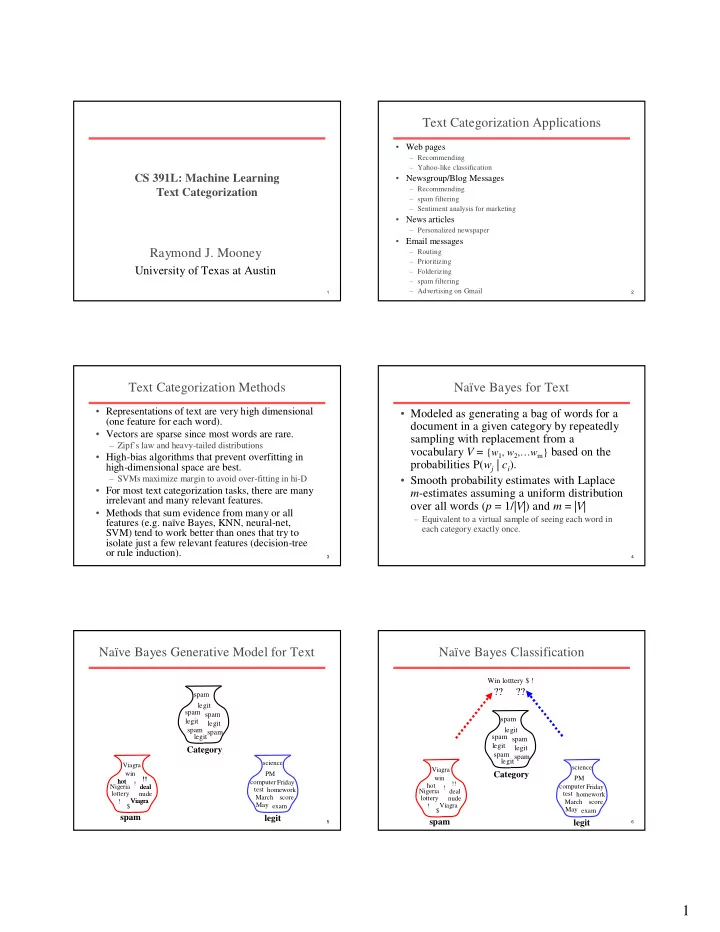
Naïve Bayes Generative Model for Text

spam legit

hot $Viagra lottery !! ! win Friday exam computer May PM test March science Viagra homework score ! spam legit spam spam legit spam legit legitspam

Category

Viagra deal hot !!

6

Naïve Bayes Classification

nude deal Nigeria

spam legit

hot $Viagra lottery !! ! win Friday exam computer May PM test March science Viagra homework score ! spam legit spam spam legit spam legit legitspam

Category

Win lotttery $ !

?? ??

2

7

Text Naïve Bayes Algorithm (Train)

Let V be the vocabulary of all words in the documents in D For each category ci ∈ C Let Di be the subset of documents in D in category ci P(ci) = |Di| / |D| Let Ti be the concatenation of all the documents in Di Let ni be the total number of word occurrences in Ti For each word wj ∈ V Let nij be the number of occurrences of wj in Ti Let P(wj | ci) = (nij + 1) / (ni + |V|)

8

Text Naïve Bayes Algorithm (Test)

Given a test document X Let n be the number of word occurrences in X Return the category: where ai is the word occurring the ith position in X ) | ( ) ( argmax

1

∏

= ∈ n i i i i C i c

c a P c P

9

Underflow Prevention

• Multiplying lots of probabilities, which are

between 0 and 1 by definition, can result in floating-point underflow.

• Since log(xy) = log(x) + log(y), it is better to

perform all computations by summing logs

• f probabilities rather than multiplying

probabilities.

• Class with highest final un-normalized log

probability score is still the most probable.

10

Naïve Bayes Posterior Probabilities

• Classification results of naïve Bayes (the

class with maximum posterior probability) are usually fairly accurate.

• However, due to the inadequacy of the

conditional independence assumption, the actual posterior-probability numerical estimates are not.

– Output probabilities are generally very close to 0 or 1.

11

Textual Similarity Metrics

• Measuring similarity of two texts is a well-studied

problem.

• Standard metrics are based on a “bag of words”

model of a document that ignores word order and syntactic structure.

• May involve removing common “stop words” and

stemming to reduce words to their root form.

• Vector-space model from Information Retrieval

(IR) is the standard approach.

• Other metrics (e.g. edit-distance) are also used.

12

The Vector-Space Model

• Assume t distinct terms remain after preprocessing;

call them index terms or the vocabulary.

• These “orthogonal” terms form a vector space.

Dimension = t = |vocabulary|

• Each term, i, in a document or query, j, is given a

real-valued weight, wij.

• Both documents and queries are expressed as

t-dimensional vectors:

dj = (w1j, w2j, …, wtj)

3

13

Graphic Representation

Example: D1 = 2T1 + 3T2 + 5T3 D2 = 3T1 + 7T2 + T3 Q = 0T1 + 0T2 + 2T3 T3 T1 T2 D1 = 2T1+ 3T2 + 5T3 D2 = 3T1 + 7T2 + T3 Q = 0T1 + 0T2 + 2T3

7 3 2 5

• Is D1 or D2 more similar to Q?
• How to measure the degree of

similarity? Distance? Angle? Projection?

14

Document Collection

• A collection of n documents can be represented in the

vector space model by a term-document matrix.

• An entry in the matrix corresponds to the “weight” of a

term in the document; zero means the term has no significance in the document or it simply doesn’t exist in the document. T1 T2 …. Tt D1 w11 w21 … wt1 D2 w12 w22 … wt2 : : : : : : : : Dn w1n w2n … wtn

15

Term Weights: Term Frequency

• More frequent terms in a document are more

important, i.e. more indicative of the topic. fij = frequency of term i in document j

• May want to normalize term frequency (tf) by

dividing by the frequency of the most common term in the document: tfij = fij / maxi{fij}

16

Term Weights: Inverse Document Frequency

• Terms that appear in many different documents

are less indicative of overall topic. df i = document frequency of term i = number of documents containing term i idfi = inverse document frequency of term i, = log2 (N/ df i) (N: total number of documents)

• An indication of a term’s discrimination power.
• Log used to dampen the effect relative to tf.

17

TF-IDF Weighting

• A typical combined term importance indicator is

tf-idf weighting: wij = tfij idfi = tfij log2 (N/ dfi)

• A term occurring frequently in the document but

rarely in the rest of the collection is given high weight.

• Many other ways of determining term weights

have been proposed.

• Experimentally, tf-idf has been found to work well.

18

Cosine Similarity Measure

• Cosine similarity measures the cosine of

the angle between two vectors.

• Inner product normalized by the vector

lengths.

D1 = 2T1 + 3T2 + 5T3 CosSim(D1 , Q) = 10 / √(4+9+25)(0+0+4) = 0.81 D2 = 3T1 + 7T2 + 1T3 CosSim(D2 , Q) = 2 / √(9+49+1)(0+0+4) = 0.13 Q = 0T1 + 0T2 + 2T3 θ2 t3 t1 t2

D1 D2 Q

θ1 D1 is 6 times better than D2 using cosine similarity but only 5 times better using inner product.

∑ ∑ ∑

= = =

• ⋅

⋅ = ⋅

t i t i t i

w w w w q d q d

iq ij iq ij j j

1 1 2 2 1

) (

r r r r

CosSim(dj, q) =

4

19

Relevance Feedback in IR

• After initial retrieval results are presented,

allow the user to provide feedback on the relevance of one or more of the retrieved documents.

• Use this feedback information to reformulate

the query.

• Produce new results based on reformulated

query.

• Allows more interactive, multi-pass process.

20

Relevance Feedback Architecture

Rankings

IR System Document corpus Ranked Documents

• 1. Doc1
• 2. Doc2
• 3. Doc3

. .

• 1. Doc1 ⇓
• 2. Doc2 ⇑
• 3. Doc3 ⇓

. .

Feedback Query String Revised Query ReRanked Documents

• 1. Doc2
• 2. Doc4
• 3. Doc5

. .

Query Reformulation

21

Using Relevance Feedback (Rocchio)

• Relevance feedback methods can be adapted for

text categorization.

• Use standard TF/IDF weighted vectors to

represent text documents (normalized by maximum term frequency).

• For each category, compute a prototype vector by

summing the vectors of the training documents in the category.

• Assign test documents to the category with the

closest prototype vector based on cosine similarity.

22

Illustration of Rocchio Text Categorization

23

Rocchio Text Categorization Algorithm (Training)

Assume the set of categories is {c1, c2,…cn} For i from 1 to n let pi = <0, 0,…,0> (init. prototype vectors) For each training example <x, c(x)> ∈ D Let d be the frequency normalized TF/IDF term vector for doc x Let i = j: (cj = c(x)) (sum all the document vectors in ci to get pi) Let pi = pi + d

24

Rocchio Text Categorization Algorithm (Test)

Given test document x Let d be the TF/IDF weighted term vector for x Let m = –2 (init. maximum cosSim) For i from 1 to n: (compute similarity to prototype vector) Let s = cosSim(d, pi) if s > m let m = s let r = ci (update most similar class prototype) Return class r

5

25

Rocchio Properties

• Does not guarantee a consistent hypothesis.
• Forms a simple generalization of the

examples in each class (a prototype).

• Prototype vector does not need to be

averaged or otherwise normalized for length since cosine similarity is insensitive to vector length.

• Classification is based on similarity to class

prototypes.

26

Rocchio Anomoly

• Prototype models have problems with

polymorphic (disjunctive) categories.

27

Illustration of 3 Nearest Neighbor for Text

28

K Nearest Neighbor for Text

Training: For each each training example <x, c(x)> ∈ D Compute the corresponding TF-IDF vector, dx, for document x Test instance y: Compute TF-IDF vector d for document y For each <x, c(x)> ∈ D Let sx = cosSim(d, dx) Sort examples, x, in D by decreasing value of sx Let N be the first k examples in D. (get most similar neighbors) Return the majority class of examples in N

29

3 Nearest Neighbor Comparison

• Nearest Neighbor tends to handle

polymorphic categories well.

30

Inverted Index

• Linear search through training texts is not

scalable.

• An index that points from words to

documents that contain them allows more rapid retrieval of similar documents.

• Once stop-words are eliminated, the

remaining words are rare, so an inverted index narrows attention to a relatively small number of documents that share meaningful vocabulary with the test document.

6

31

Conclusions

• Many important applications of

classification to text.

• Requires an approach that works well with

large, sparse features vectors, since typically each word is a feature and most words are rare.

– Naïve Bayes – kNN with cosine similarity – SVMs