1 Optimality Summary What is Search For? Tree search: Models of - - PDF document

1

Introduction to Artificial Intelligence

V22.0472-001 Fall 2009 Lecture 4: Constraint Lecture 4: Constraint Satisfaction Problems

Rob Fergus – Dept of Computer Science, Courant Institute, NYU Many slides from Dan Klein, Stuart Russell or Andrew Moore

Announcements

• Please ask for help on assignment

2

Today

• Search Conclusion

C S f P bl

• Constraint Satisfaction Problems

A* Review

• A* uses both backward costs g and forward estimate

h: f(n) = g(n) + h(n)

• A* tree search is optimal with admissible heuristics

p (optimistic future cost estimates)

• Heuristic design is key: relaxed problems can help

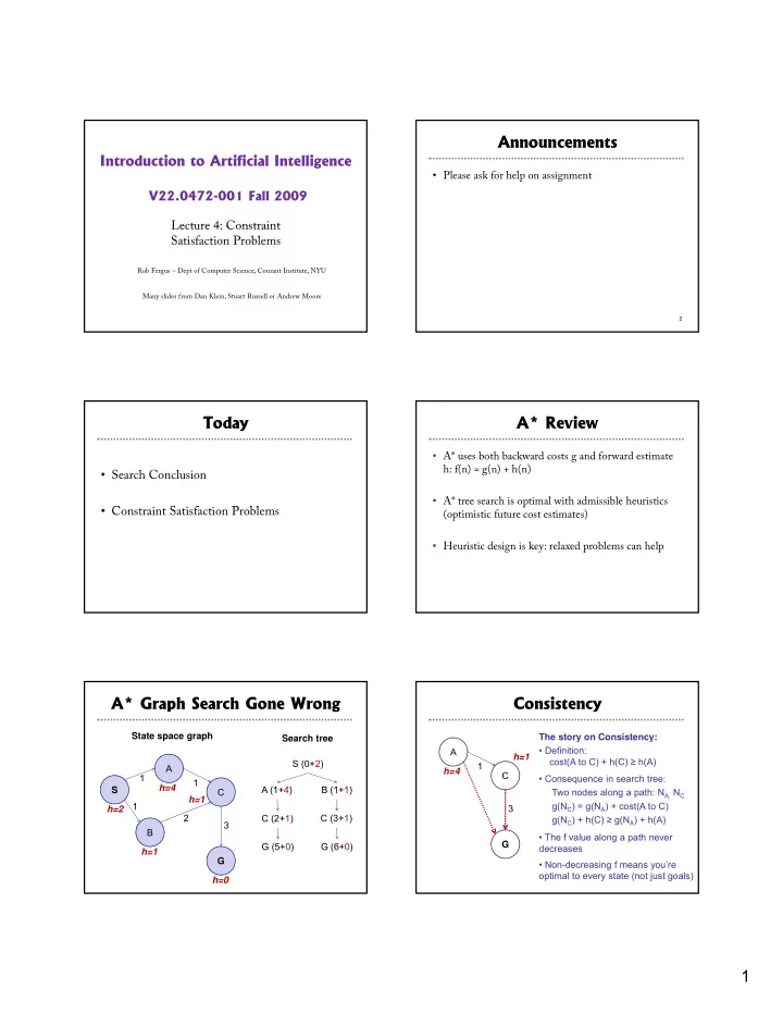
A* Graph Search Gone Wrong

S A 1 1 h=4 S (0+2) A (1 4) B (1 1) S A State space graph Search tree S B C G 1 2 3 h=2 h=1 h=4 h=1 h=0 A (1+4) B (1+1) C (2+1) G (5+0) C (3+1) G (6+0) S B C G

Consistency

A C h=4 h=1 1 The story on Consistency:

• Definition:

cost(A to C) + h(C) ≥ h(A)

• Consequence in search tree:

3 G Two nodes along a path: NA, NC g(NC) = g(NA) + cost(A to C) g(NC) + h(C) ≥ g(NA) + h(A)

• The f value along a path never

decreases

• Non-decreasing f means you’re
• ptimal to every state (not just goals)

2

Optimality Summary

• Tree search:
• A* optimal if heuristic is admissible (and non-negative)
• Uniform Cost Search is a special case (h = 0)
• Graph search:

p

• A* optimal if heuristic is consistent
• UCS optimal (h = 0 is consistent)
• In general, natural admissible heuristics tend to be

consistent

• Remember, costs are always positive in search!

What is Search For?

• Models of the world: single agents, deterministic actions, fully
• bserved state, discrete state space
• Planning: sequences of actions
• The path to the goal is the important thing
• The path to the goal is the important thing
• Paths have various costs, depths
• Heuristics to guide, fringe to keep backups
• Identification: assignments to variables
• The goal itself is important, not the path
• All paths at the same depth (for some formulations)
• CSPs are specialized for identification problems

8

Constraint Satisfaction Problems

• Standard search problems:
• State is a “black box”: arbitrary data structure
• Goal test: any function over states
• Successor function can be anything
• Constraint satisfaction problems (CSPs):
• A special subset of search problems

A special subset of search problems

• State is defined by variables Xi with values from a

domain D (sometimes D depends on i)

• Goal test is a set of constraints specifying allowable

combinations of values for subsets of variables

• Simple example of a formal representation language
• Allows useful general-purpose algorithms with more

power than standard search algorithms

9

Example: N-Queens

• Formulation 1:
• Variables:
• Domains:
• Constraints

Constraints

10

Example: N-Queens

• Formulation 1.5:
• Variables:
• Domains:

Domains:

• Constraints:

… there’s an even better way! What is it?

Example: N-Queens

• Formulation 2:
• Variables:
• Domains:

Domains:

• Constraints:

Implicit: Explicit:

• or-

3

Example: Map-Coloring

• Variables:
• Domain:
• Constraints: adjacent regions must have

different colors

• Solutions are assignments satisfying all

constraints, e.g.:

13

Constraint Graphs

• Binary CSP: each constraint

relates (at most) two variables

• Binary constraint graph: nodes are

variables, arcs show constraints

• General-purpose CSP algorithms

use the graph structure to speed up

• search. E.g., Tasmania is an

independent subproblem!

14

Example: Cryptarithmetic

• Variables (circles):
• Domains:
• Constraints (boxes):

15

Example: Sudoku

Variables: Each (open) square Domains: Domains: {1,2,…,9} Constraints:

9-way alldiff for each row 9-way alldiff for each column 9-way alldiff for each region

Example: The Waltz Algorithm

• The Waltz algorithm is for interpreting line drawings of solid

polyhedra

• An early example of a computation posed as a CSP
• Look at all intersections
• Adjacent intersections impose constraints on each other

?

17

Waltz on Simple Scenes

• Assume all objects:
• Have no shadows or cracks
• Three-faced vertices
• “General position”: no junctions

change with small movements of the eye eye.

• Then each line on image is one of

the following:

• Boundary line (edge of an object)

(→) with right hand of arrow denoting “solid” and left hand denoting “space”

• Interior convex edge (+)
• Interior concave edge (-)

18

4

Legal Junctions

• Only certain junctions are physically

possible

• How can we formulate a CSP to

label an image?

• Variables: vertices
• Domains: junction labels
• Constraints: both ends of a line

should have the same label

x y (x,y) in

, , …

19

Varieties of CSPs

• Discrete Variables
• Finite domains
• Size d means O(dn) complete assignments
• E.g., Boolean CSPs, including Boolean satisfiability (NP-complete)
• Infinite domains (integers, strings, etc.)
• E g job scheduling variables are start/end times for each job
• E.g., job scheduling, variables are start/end times for each job
• Linear constraints solvable, nonlinear undecidable
• Continuous variables
• E.g., start/end times for Hubble Telescope observations
• Linear constraints solvable in polynomial time by LP methods (see

cs170 for a bit of this theory)

20

Varieties of Constraints

• Varieties of Constraints
• Unary constraints involve a single variable (equiv. to shrinking domains):
• Binary constraints involve pairs of variables:
• Higher-order constraints involve 3 or more variables:

e.g., cryptarithmetic column constraints

• Preferences (soft constraints):
• E.g., red is better than green
• Often representable by a cost for each variable assignment
• Gives constrained optimization problems
• (We’ll ignore these until we get to Bayes’ nets)

21

Real-World CSPs

• Assignment problems: e.g., who teaches what class
• Timetabling problems: e.g., which class is offered when and

where?

• Hardware configuration
• Transportation scheduling

p g

• Factory scheduling
• Floorplanning
• Fault diagnosis
• … lots more!
• Many real-world problems involve real-valued variables…

22

Standard Search Formulation

• Standard search formulation of CSPs (incremental)
• Let's start with the straightforward, dumb approach, then fix it
• States are defined by the values assigned so far

y g

• Initial state: the empty assignment, {}
• Successor function: assign a value to an unassigned variable
• Goal test: the current assignment is complete and satisfies all

constraints

• Simplest CSP ever: two bits, constrained to be equal

23

Search Methods

• What does BFS do?
• What does DFS do?

What does DFS do?

• What’s the obvious problem here?
• What’s the slightly-less-obvious problem?

24

5

Backtracking Search

• Idea 1: Only consider a single variable at each point
• Variable assignments are commutative, so fix ordering
• I.e., [WA = red then NT = green] same as [NT = green then WA = red]
• Only need to consider assignments to a single variable at each step
• How many leaves are there?
• Idea 2: Only allow legal assignments at each point

y g g p

• I.e. consider only values which do not conflict previous assignments
• Might have to do some computation to figure out whether a value is ok
• “Incremental goal test”
• Depth-first search for CSPs with these two improvements is called

backtracking search

• Backtracking search is the basic uninformed algorithm for CSPs
• Can solve n-queens for n ≈ 25

25

Backtracking Search

• What are the choice points?

26

Backtracking Example

27

Improving Backtracking

• General-purpose ideas can give huge gains in speed:
• Which variable should be assigned next?
• In what order should its values be tried?
• Can we detect inevitable failure early?
• Can we take advantage of problem structure?

28

Minimum Remaining Values

• Minimum remaining values (MRV):
• Choose the variable with the fewest legal values
• Why min rather than max?
• Also called “most constrained variable”
• “Fail-fast” ordering

29

Degree Heuristic

• Tie-breaker among MRV variables
• Degree heuristic:
• Choose the variable participating in the most constraints
• n remaining variables
• Why most rather than fewest constraints?

30

6

Least Constraining Value

• Given a choice of variable:
• Choose the least constraining value
• The one that rules out the fewest

values in the remaining variables

• Note that it may take some

computation to determine this! p

• Why least rather than most?
• Combining these heuristics

makes 1000 queens feasible

31

Forward Checking

• Idea: Keep track of remaining legal values for unassigned

variables (using immediate constraints)

• Idea: Terminate when any variable has no legal values

WA SA NT Q

NSW

V 32

Constraint Propagation

• Forward checking propagates information from assigned to adjacent

unassigned variables, but doesn't detect more distant failures:

WA SA NT Q

NSW

V

• NT and SA cannot both be blue!
• Why didn’t we detect this yet?
• Constraint propagation repeatedly enforces constraints (locally)

33

Arc Consistency

• Simplest form of propagation makes each arc consistent
• X → Y is consistent iff for every value x there is some allowed y

WA SA NT Q

NSW

V 34

• If X loses a value, neighbors of X need to be rechecked!
• Arc consistency detects failure earlier than forward checking
• What’s the downside of arc consistency?
• Can be run as a preprocessor or after each assignment

Arc Consistency

• Runtime: O(n2d3), can be reduced to O(n2d2)
• … but detecting all possible future problems is NP-hard – why?

35

Limitations of Arc Consistency

• After running arc

consistency:

• Can have one solution left
• Can have multiple solutions

l f left

• Can have no solutions left

(and not know it)

7

Problem Structure

• Tasmania and mainland are independent

subproblems

• Identifiable as connected components of

constraint graph

• Suppose each subproblem has c variables
• ut of n total
• Worst-case solution cost is O((n/c)(dc)),

linear in n

• E.g., n = 80, d = 2, c =20
• 280 = 4 billion years at 10 million nodes/sec
• (4)(220) = 0.4 seconds at 10 million nodes/sec

37

Tree-Structured CSPs

• Choose a variable as root, order

variables from root to leaves such that every node's parent precedes it in the ordering

• For i = n : 2, apply RemoveInconsistent(Parent(Xi),Xi)
• For i = 1 : n, assign Xi consistently with Parent(Xi)
• Runtime: O(n d2)

38

Tree-Structured CSPs

• Theorem: if the constraint graph has no loops, the CSP can be solved in

O(n d2) time!

• Compare to general CSPs, where worst-case time is O(dn)
• This property also applies to logical and probabilistic reasoning: an

important example of the relation between syntactic restrictions and the complexity of reasoning.

39

Nearly Tree-Structured CSPs

• Conditioning: instantiate a variable, prune its neighbors' domains
• Cutset conditioning: instantiate (in all ways) a set of variables such that the

remaining constraint graph is a tree

• Cutset size c gives runtime O( (dc) (n-c) d2 ), very fast for small c

40

Iterative Algorithms for CSPs

• Greedy and local methods typically work with “complete”

states, i.e., all variables assigned

• To apply to CSPs:
• Allow states with unsatisfied constraints
• Operators reassign variable values

Operators reassign variable values

• Variable selection: randomly select any conflicted variable
• Value selection by min-conflicts heuristic:
• Choose value that violates the fewest constraints
• I.e., hill climb with h(n) = total number of violated constraints

41

Example: 4-Queens

• States: 4 queens in 4 columns (44 = 256 states)
• Operators: move queen in column
• Goal test: no attacks
• Evaluation: h(n) = number of attacks

42

8

Performance of Min-Conflicts

• Given random initial state, can solve n-queens in almost constant time for

arbitrary n with high probability (e.g., n = 10,000,000)

• The same appears to be true for any randomly-generated CSP except in a

narrow range of the ratio

43

Summary

• CSPs are a special kind of search problem:
• States defined by values of a fixed set of variables
• Goal test defined by constraints on variable values
• Backtracking = depth-first search with one legal variable assigned per node
• Variable ordering and value selection heuristics help significantly
• Forward checking prevents assignments that guarantee later failure
• Constraint propagation (e.g., arc consistency) does additional work to constrain values and

detect inconsistencies

• The constraint graph representation allows analysis of problem structure
• Tree-structured CSPs can be solved in linear time
• Iterative min-conflicts is usually effective in practice

44

Node Class

class Node: def __init__(self, state, parent, action, path_cost): "Create a search tree Node, derived from a parent by an action." “YOUR CODE HERE: Set state, parent, action, path_cost" self.state = state etc……. if parent: “YOUR CODE HERE: If valid parent, increment depth, path_cost” def path(self): "Create a list of nodes from the root to this node." “ i.e. Follow parent pointers back up to root” def expand(self, problem): "Return a list of nodes reachable from this node" return [Node(next, self, act, path_cost) for (next, act, path_cost) in problem.getSuccessors(self.state)]

Graph Search

def graph_search(problem, fringe): "Search through the successors of a problem to find a goal.” return None def depthFirstSearch(problem): def depthFirstSearch(problem): “Search the deepest nodes in the search tree first” return graph_search(problem, util.Stack()) def breadthFirstSearch(problem): "Search the shallowest nodes in the search tree first” return graph_search(problem, util.Queue())