1 2.1 Mobility trees Mobility tree, Men Working status 04 - - PDF document

SLIDE 1

✬ ✫ ✩ ✪

IPUC, Neuchˆ atel, February 23-24, 2007

Innovative Data Mining based approaches for life course analysis

Gilbert Ritschard Alexis Gabadinho, Nicolas M¨ uller, Matthias Studer University of Geneva, Switzerland

Outline 1 Aim of the research project 2 Our first results 2.1 Mobility trees 2.2 Survival trees 2.3 Characteristic sequences 3 Foreseen Developments

http://mephisto.unige.ch IPUC07 toc intro mob surv seq conc ◭ ◮ 22/2/2007gr 1

✬ ✫ ✩ ✪

1 Aim of the research project

Just started February 1, 2007 FNS project on “Mining event histories: Towards new insight on personal Swiss life courses” Methodological concern Explore and develop data mining approaches for individual longitudinal data

• Methods for time to event analysis
• Methods for sequence data analysis

Socio-demographic concern Using mainly SHP data, but also other sources, gain original insight on

• How familial, professional and other socio-demographic events are

entwined,

• Typical characteristics of Swiss life trajectories,
• Changes in these characteristics over time.

IPUC07 toc intro mob surv seq conc ◭ ◮ 22/2/2007gr 2

✬ ✫ ✩ ✪

What is data mining?

“Data Mining is the process of finding new and potentially useful knowledge from data” Gregory Piatetsky-Shapiro editor of http://www.kdnuggets.com “Data mining is the analysis of (often large) observational data sets to find unsuspected relationships and to summarize the data in novel ways that are both understandable and useful to the data owner” (Hand et al., 2001) Also called Knowledge Discovery in Databases, KDD. Origin: IJCAI Workshop, 1989, Piatetsky-Shapiro (1989) Textbooks : Han and Kamber (2001), Hand et al. (2001)

IPUC07 toc intro mob surv seq conc ◭ ◮ 22/2/2007gr 3

✬ ✫ ✩ ✪

What is data mining? (2)

Concerned with characterization of interesting patterns

• per se (unsupervised learning)

– Clustering – Frequent itemsets – Association rules

• for classification or prediction purposes (supervised learning)

– Decision trees – Bayesian networks – SVM and Kernel Methods – CBR (case based reasoning), K-NN (k nearest neighbors) Proceeds mainly heuristically . Unlike statistical modeling, makes no assumptions about process generating the data.

IPUC07 toc intro mob surv seq conc ◭ ◮ 22/2/2007gr 4

✬ ✫ ✩ ✪

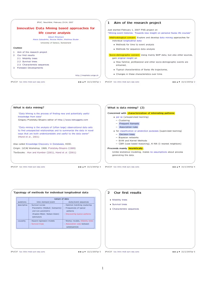
Typology of methods for individual longitudinal data

nature of data questions time stamped event state/event sequences descriptive

• Survival curves:
• Optimal matching clustering

Parametric (Weibull, Gompertz)

• Frequencies of typical

and non parametric patterns (Kaplan-Meier, Nelson-Aalen)

• Discovering typical patterns

estimators causality

• Hazard regression models
• Markov models, Mobility trees
• Survival trees
• Association rules between

subsequences IPUC07 toc intro mob surv seq conc ◭ ◮ 22/2/2007gr 5

✬ ✫ ✩ ✪

2 Our first results

• Mobility trees
• Survival trees
• Characteristic sequences

IPUC07 toc intro mob surv seq conc ◭ ◮ 22/2/2007gr 6

1

SLIDE 2

✬ ✫ ✩ ✪

2.1 Mobility trees

• (SHP Data, Waves 1 to 6 (1999-2004), aged between 20 and 64 in 2004.)
• How does working status (occupied active, unemployed, inactive) in 2004

depend on – working status in previous year (1999 to 2003) – other factors (attained education level, partner working status, partner education level, ...) and what are main interaction effects?

• Mobility trees are alternative to Markovian transition models.
• Growing separate classification trees for women and men highlights

gender differences.

IPUC07 toc intro mob surv seq conc ◭ ◮ 22/2/2007gr 7

✬ ✫ ✩ ✪ Mobility tree, Men

Category % n active occupied 93.06 1194 unemployed 1.56 20 not in labor force 5.38 69 Total (100.00) 1283 Node 0 Category % n active occupied 82.48 113 unemployed 5.84 8 not in labor force 11.68 16 Total (10.68) 137 Node 3 Category % n active occupied 70.13 54 unemployed 10.39 8 not in labor force 19.48 15 Total (6.00) 77 Node 7 Category % n active occupied 98.33 59 unemployed 0.00 not in labor force 1.67 1 Total (4.68) 60 Node 6 Category % n active occupied 29.51 18 unemployed 4.92 3 not in labor force 65.57 40 Total (4.75) 61 Node 2 Category % n active occupied 97.97 1063 unemployed 0.83 9 not in labor force 1.20 13 Total (84.57) 1085 Node 1 Category % n active occupied 95.19 356 unemployed 1.87 7 not in labor force 2.94 11 Total (29.15) 374 Node 5 Category % n active occupied 99.44 707 unemployed 0.28 2 not in labor force 0.28 2 Total (55.42) 711 Node 4 Working status 04 Working status B, 03

• Adj. P-value=0.0000, Chi-square=240.3194, df=2

unemployed,<missing> Partner actual occupation 04, into 6

• Adj. P-value=0.0002, Chi-square=20.7799, df=1

education,<missing> at home;part-time paid w ork;full time paid w ork + family company;retired or invalid not in labour force active, full time (>= 80%);active, long part time (50%-80%);active, short part time (< 50%) Partner highest level of education achieved 04 (both grid and individual quest.)

• Adj. P-value=0.0001, Chi-square=20.7372, df=1

>vocational high school,<missing> <=vocational high school

IPUC07 toc intro mob surv seq conc ◭ ◮ 22/2/2007gr 8

✬ ✫ ✩ ✪ Mobility tree, Women

Category % n active occupied 77.78 1281 unemployed 2.31 38 not in labor force 19.91 328 Total (100.00) 1647 Node 0 Category % n active occupied 73.33 143 unemployed 7.69 15 not in labor force 18.97 37 Total (11.84) 195 Node 4 Category % n active occupied 87.50 77 unemployed 5.68 5 not in labor force 6.82 6 Total (5.34) 88 Node 12 Category % n active occupied 61.68 66 unemployed 9.35 10 not in labor force 28.97 31 Total (6.50) 107 Node 11 Category % n active occupied 91.78 346 unemployed 0.80 3 not in labor force 7.43 28 Total (22.89) 377 Node 3 Category % n active occupied 94.98 303 unemployed 0.31 1 not in labor force 4.70 15 Total (19.37) 319 Node 10 Category % n active occupied 74.14 43 unemployed 3.45 2 not in labor force 22.41 13 Total (3.52) 58 Node 9 Category % n active occupied 95.69 733 unemployed 1.17 9 not in labor force 3.13 24 Total (46.51) 766 Node 2 Category % n active occupied 89.26 133 unemployed 2.68 4 not in labor force 8.05 12 Total (9.05) 149 Node 8 Category % n active occupied 97.24 600 unemployed 0.81 5 not in labor force 1.94 12 Total (37.46) 617 Node 7 Category % n active occupied 99.25 265 unemployed 0.37 1 not in labor force 0.37 1 Total (16.21) 267 Node 14 Category % n active occupied 95.71 335 unemployed 1.14 4 not in labor force 3.14 11 Total (21.25) 350 Node 13 Category % n active occupied 19.09 59 unemployed 3.56 11 not in labor force 77.35 239 Total (18.76) 309 Node 1 Category % n active occupied 39.73 29 unemployed 9.59 7 not in labor force 50.68 37 Total (4.43) 73 Node 6 Category % n active occupied 12.71 30 unemployed 1.69 4 not in labor force 85.59 202 Total (14.33) 236 Node 5 Working status 04 Working status B, 03

• Adj. P-value=0.0000, Chi-square=750.9194, df=3

unemployed,<missing> Working status B, 00

• Adj. P-value=0.0004, Chi-square=19.1782, df=1

active, full time (>= 80%);active, short part time (< 50%) not in labour force;unemployed;active, long part time (50%-80%),<missing> active, short part time (< 50%) Working status B, 02

• Adj. P-value=0.0003, Chi-square=19.3525, df=1

active, short part time (< 50%);unemployed;active, long part time (50%-80%),<missing> not in labour force;active, full time (>= 80%) active, full time (>= 80%);active, long part time (50%-80%) Working status B, 99

• Adj. P-value=0.0047, Chi-square=14.3681, df=1

not in labour force;unemployed,<missing> active, full time (>= 80%);active, long part time (50%-80%);active, short part time (< 50%) Highest level of education achieved 04 (both grid and individual quest.)

• Adj. P-value=0.0292, Chi-square=8.6618, df=1

>full-time vocational school <=full-time vocational school not in labour force Working status B, 02

• Adj. P-value=0.0000, Chi-square=30.5767, df=1

active, full time (>= 80%);active, short part time (< 50%);unemployed;active, long part time (50%-80%),<missing> not in labour force

Working status B (full time, long part time, short part time, unemployed, inactive) in 2003 used for first split

IPUC07 toc intro mob surv seq conc ◭ ◮ 22/2/2007gr 9

✬ ✫ ✩ ✪ Mobility tree, Women: Details for women inactive in 2003

Category % n active occupied 19.09 59 unemployed 3.56 11 not in labor force 77.35 239 Total (18.76) 309 Node 1 Category % n active occupied 39.73 29 unemployed 9.59 7 not in labor force 50.68 37 Total (4.43) 73 Node 6 Category % n active occupied 12.71 30 unemployed 1.69 4 not in labor force 85.59 202 Total (14.33) 236 Node 5 not in labour force Working status B, 02

• Adj. P-value=0.0000, Chi-square=30.5767, df=1

active, full time (>= 80%);active, short part time (< 50%);unemployed;active, long part time (50%-80%),<missing> not in labour force

IPUC07 toc intro mob surv seq conc ◭ ◮ 22/2/2007gr 10

✬ ✫ ✩ ✪

2.2 Survival trees

• (SHP 2002 biographical data, 2002 Wave data for some potential explanatory factors)
• Which are the most discriminating factors for marriage duration until

divorce/separation? Used same variables as for discrete time logistic model in Ritschard and

Sauvain-Dugerdil (2007)

• Tried two methods

– Maximize differences in KM survival curves using Tarone-Ware (T-W) p-value (Segal, 1988). – Cox regression tree: maximize differences in proportionality factors among groups (Leblanc and Crowley, 1992; Therneau and Atkinson, 1997)

IPUC07 toc intro mob surv seq conc ◭ ◮ 22/2/2007gr 11

✬ ✫ ✩ ✪ T-W Survival Tree: Marriage until Divorce/Separation

Population n = 3619, e = 622 S < 90% at 11 S at 30 = 0.77 TW χ2(1) = 54.81, p<0.0001 <=1940 n = 841, e = 123 S < 90% at 21 S at 30 = 0.86 TW χ2(1) = 22.48, p<0.0001 > 1940 n =2778, e = 499 S <90% at 9 S at 30 = 0.73 TW χ2(1) = 37.44, p<0.0001 <=1940 & French L. n = 174, e = 44 S < 90% at 11 S at 30 = 0.74 <=1940 & Non French L. n = 667, e = 79 S < 90% at 26 S at 30 = 0.89 TW χ2(1) = 8.08, p<0.0001 > 1940 & No Child n = 603, e = 138 S < 90% at 5 S at 30 = 0.64 TW χ2(1) = 4.45, p=0.0349 > 1940 & Child n = 2175, e = 361 S < 90% at 11 S at 30 = 0.75 TW χ2(1) = 9.77, p=0.0018 > 1940 & Child & German or Italian L. n = 1444, e = 217 S < 90% at 13 S at 30 = 0.77 > 1940 & Child & French or unknown L. n =731, e = 144 S < 90% at 8 S at 30 = 0.70 <=1940 & Non French L. & University n = 51, e = 12 S < 90% at 10 S at 30 = 0.76 <=1940 & Non French L. & Not University n = 667, e = 79 S < 90% at 29 S at 30 = 0.895 > 1940 & No Child & University n = 86, e = 23 S < 90% at 3 S at 30 = 0.59 > 1940 & No Child & Not University n = 517, e = 138 S < 90% at 6 S at 30 = 0.65

IPUC07 toc intro mob surv seq conc ◭ ◮ 22/2/2007gr 12

2

SLIDE 3

✬ ✫ ✩ ✪

10 20 30 40 0.5 0.6 0.7 0.8 0.9 1.0 Noeud finaux Cohorte <=1940 et Allemand, Italien ou inconnu et Université Cohorte <=1940 et Langue Allemand, Italien ou inconnu et Non Université Cohorte <=1940 et Langue Français Cohorte > 1940 et Sans Enfant et Universitaire Cohorte > 1940 et Sans Enfant et Non Universitaire Cohorte > 1940 et Avec Enfant et (Allemand ou Italien) Cohorte > 1940 et Avec Enfant et (Français ou Inconnu)

IPUC07 toc intro mob surv seq conc ◭ ◮ 22/2/2007gr 13

✬ ✫ ✩ ✪ Marriage survival probabilities until Divorce/Separation, by leaves

0.1 0.2 0.3 0.4 0.5 0.6 0.7 0.8 0.9 1

<=1940 & non French L. & University <=1940 & non French L. & non University <=1940 & French L. > 1940 & no Child & University > 1940 & no Child & non University > 1940 & Child & German or Italian L. > 1940 & Child & French or unknown L.

Survival probability 5 years 10 years 20 years 30 years IPUC07 toc intro mob surv seq conc ◭ ◮ 22/2/2007gr 14

✬ ✫ ✩ ✪ Cox Survival Tree: Marriage until Divorce/Separation

Population n = 3619, e = 622

• Prop. fact. = 1.0
• LL improv.= 55.87

<=1940 n = 841, e = 123

• Prop. fact. = 0.60
• LL improv.= 18.44

> 1940 n = 2778, e = 499

• Prop. fact. = 1.20
• LL improv.= 30.91

<=1940 & French n = 174, e = 44

• Prop. fact. = 1.10

<=1940 & Non French n = 667, e = 79

• Prop. fact. = 0.48

> 1940 & No Child n = 603, e = 138

• Prop. fact. = 1.88

> 1940 & Child n = 2175, e = 361

• Prop. fact. = 1.06

IPUC07 toc intro mob surv seq conc ◭ ◮ 22/2/2007gr 15

✬ ✫ ✩ ✪

10 20 30 40 0.5 0.6 0.7 0.8 0.9 1.0

Noeud finaux

Cohorte <=1940 et Langue Allemand, Italien ou inconnu Cohorte <=1940 et Langue Français Cohorte > 1940 et Avec Enfant Cohorte > 1940 et Sans Enfant

IPUC07 toc intro mob surv seq conc ◭ ◮ 22/2/2007gr 16

✬ ✫ ✩ ✪

2.3 Characteristic sequences

• (SHP 2002 biographical data)
• Selection of pairs of events, e.g. marriage and first job.
• For each pair, order of sequence: <, =, >, missing
• Which are the most typical sequences?
• Most discriminating sequences between

– sex – birth cohort (1940 and before, after 1940)

IPUC07 toc intro mob surv seq conc ◭ ◮ 22/2/2007gr 17

✬ ✫ ✩ ✪ Frequencies of characteristic 2-event sequences

0% 5% 10% 15% 20% 25% 30% C h i l d < M a r r i a g e M a r r i a g e < C h i l d C h i l d = M a r r i a g e C h i l d < J

• b

J

• b

< C h i l d C h i l d = J

• b

C h i l d < E d u c e n d E d u c e n d < C h i l d C h i l d = E d u c e n d M a r r i a g e < J

• b

J

• b

< M a r r i a g e M a r r i a g e = J

• b

M a r r i a g e < E d u c e n d E d u c e n d < M a r r i a g e M a r r i a g e = E d u c e n d J

• b

< E d u c e n d E d u c e n d < J

• b

J

• b

= E d u c e n d IPUC07 toc intro mob surv seq conc ◭ ◮ 22/2/2007gr 18

3

SLIDE 4

✬ ✫ ✩ ✪ Cohort discriminating 2-event sequences

Category % n apres 41 79.98 3803 avant 41 20.02 952 Total (100.00) 4755 Node 0 Category % n apres 41 84.13 1124 avant 41 15.87 212 Total (28.10) 1336 Node 4 Category % n apres 41 90.48 979 avant 41 9.52 103 Total (22.75) 1082 Node 11 Category % n apres 41 92.32 902 avant 41 7.68 75 Total (20.55) 977 Node 23 Category % n apres 41 73.33 77 avant 41 26.67 28 Total (2.21) 105 Node 22 Category % n apres 41 78.57 44 avant 41 21.43 12 Total (1.18) 56 Node 10 Category % n apres 41 51.01 101 avant 41 48.99 97 Total (4.16) 198 Node 9 Category % n apres 41 42.36 61 avant 41 57.64 83 Total (3.03) 144 Node 21 Category % n apres 41 74.07 40 avant 41 25.93 14 Total (1.14) 54 Node 20 Category % n apres 41 62.48 726 avant 41 37.52 436 Total (24.44) 1162 Node 3 Category % n apres 41 59.22 562 avant 41 40.78 387 Total (19.96) 949 Node 8 Category % n apres 41 54.43 172 avant 41 45.57 144 Total (6.65) 316 Node 19 Category % n apres 41 61.61 390 avant 41 38.39 243 Total (13.31) 633 Node 18 Category % n apres 41 76.00 164 avant 41 23.00 49 Total (4.48) 213 Node 7 Category % n apres 41 88.17 82 avant 41 11.83 11 Total (1.96) 93 Node 17 Category % n apres 41 68.33 82 avant 41 31.67 38 Total (2.52) 120 Node 16 Category % n apres 41 69.44 50 avant 41 30.56 22 Total (1.51) 72 Node 2 Category % n apres 41 87.09 1903 avant 41 12.91 282 Total (45.95) 2185 Node 1 Category % n apres 41 88.01 1688 avant 41 11.99 230 Total (40.34) 1918 Node 6 Category % n apres 41 84.82 486 avant 41 15.18 87 Total (12.05) 573 Node 15 Category % n apres 41 89.37 1202 avant 41 10.63 143 Total (28.29) 1345 Node 14 Category % n apres 41 80.52 215 avant 41 19.48 52 Total (5.62) 267 Node 5 Category % n apres 41 85.41 158 avant 41 14.59 27 Total (3.89) 185 Node 13 Category % n apres 41 69.51 57 avant 41 30.49 25 Total (1.72) 82 Node 12 Naissance Départ et mariage

• Adj. P-value=0.0000, Chi-square=310.7048, df=3

<missing> Mariage et fin des études

• Adj. P-value=0.0000, Chi-square=196.6698, df=2

<missing> Enfant et emploi

• Adj. P-value=0.0000, Chi-square=39.6959, df=1

=,<missing> >;< < >;= Enfant et emploi

• Adj. P-value=0.0007, Chi-square=15.8053, df=1

<missing> >;<;= = Départ et emploi

• Adj. P-value=0.0000, Chi-square=23.4451, df=1

>,<missing> Enfant et emploi

• Adj. P-value=0.0339, Chi-square=4.5007, df=1

<missing> > <;= Départ et fin des études

• Adj. P-value=0.0064, Chi-square=11.6421, df=1

<;= >,<missing> > < Mariage et emploi

• Adj. P-value=0.0063, Chi-square=11.6786, df=1

>;< Départ et fin des études

• Adj. P-value=0.0498, Chi-square=7.8866, df=1

=,<missing> >;< =,<missing> Départ et fin des études

• Adj. P-value=0.0249, Chi-square=9.1512, df=1

<;=,<missing> >

First split variable: {Marriage, Leaving Home}

IPUC07 toc intro mob surv seq conc ◭ ◮ 22/2/2007gr 19

✬ ✫ ✩ ✪ Cohort: details for Leaving Home before Marriage

Categor apres 41 avant 41 Total N Category % n apres 41 69.44 50 avant 41 30.56 22 Total (1.51) 72 Node 2 Category % n apres 41 87.09 1903 avant 41 12.91 282 Total (45.95) 2185 Node 1 Category % n apres 41 88.01 1688 avant 41 11.99 230 Total (40.34) 1918 Node 6 Category % n apres 41 84.82 486 avant 41 15.18 87 Total (12.05) 573 Node 15 Category % n apres 41 89.37 1202 avant 41 10.63 143 Total (28.29) 1345 Node 14 Category % n apres 41 80.52 215 avant 41 19.48 52 Total (5.62) 267 Node 5 Category % n apres 41 85.41 158 avant 41 14.59 27 Total (3.89) 185 Node 13 Category % n apres 41 69.51 57 avant 41 30.49 25 Total (1.72) 82 Node 12 Ad >,<m > < Mariage et emploi

• Adj. P-value=0.0063, Chi-square=11.6786, df=1

>;< Départ et fin des études

• Adj. P-value=0.0498, Chi-square=7.8866, df=1

=,<missing> >;< =,<missing> Départ et fin des études

• Adj. P-value=0.0249, Chi-square=9.1512, df=1

<;=,<missing> >

IPUC07 toc intro mob surv seq conc ◭ ◮ 22/2/2007gr 20

✬ ✫ ✩ ✪ Sex discriminating 2-event sequences

Category % n masculin 46.25 2199 féminin 53.75 2556 Total (100.00) 4755 Node 0 Category % n masculin 43.60 613 féminin 56.40 793 Total (29.57) 1406 Node 4 Category % n masculin 54.38 205 féminin 45.62 172 Total (7.93) 377 Node 10 Category % n masculin 39.65 408 féminin 60.35 621 Total (21.64) 1029 Node 9 Category % n masculin 63.16 36 féminin 36.84 21 Total (1.20) 57 Node 16 Category % n masculin 38.27 372 féminin 61.73 600 Total (20.44) 972 Node 15 Category % n masculin 41.32 402 féminin 58.68 571 Total (20.46) 973 Node 3 Category % n masculin 58.51 832 féminin 41.49 590 Total (29.91) 1422 Node 2 Category % n masculin 64.69 480 féminin 35.31 262 Total (15.60) 742 Node 8 Category % n masculin 76.26 196 féminin 23.74 61 Total (5.40) 257 Node 14 Category % n masculin 58.56 284 féminin 41.44 201 Total (10.20) 485 Node 13 Category % n masculin 51.76 352 féminin 48.24 328 Total (14.30) 680 Node 7 Category % n masculin 36.90 352 féminin 63.10 602 Total (20.06) 954 Node 1 Category % n masculin 21.10 23 féminin 78.90 86 Total (2.29) 109 Node 6 Category % n masculin 38.93 329 féminin 61.07 516 Total (17.77) 845 Node 5 Category % n masculin 23.81 20 féminin 76.19 64 Total (1.77) 84 Node 12 Category % n masculin 40.60 309 féminin 59.40 452 Total (16.00) 761 Node 11 sexe Emploi et fin des études

• Adj. P-value=0.0000, Chi-square=133.0423, df=3

<missing> Départ et emploi

• Adj. P-value=0.0000, Chi-square=24.3337, df=1

> <;=,<missing> Mariage et fin des études

• Adj. P-value=0.0019, Chi-square=13.9356, df=1

< >;=,<missing> = < Départ et emploi

• Adj. P-value=0.0000, Chi-square=24.4185, df=1

> Mariage et fin des études

• Adj. P-value=0.0000, Chi-square=23.0606, df=1

<;= >,<missing> <;=,<missing> > Enfant et emploi

• Adj. P-value=0.0028, Chi-square=13.1883, df=1

< >;=,<missing> Départ et fin des études

• Adj. P-value=0.0274, Chi-square=8.9750, df=1

= >;<,<missing>

First split variable: {Job, Education End}

IPUC07 toc intro mob surv seq conc ◭ ◮ 22/2/2007gr 21

✬ ✫ ✩ ✪ Sex: details for Job after Education end

Category % n masculin 36.90 352 féminin 63.10 602 Total (20.06) 954 Node 1 Category % n masculin 21.10 23 féminin 78.90 86 Total (2.29) 109 Node 6 Category % n masculin 38.93 329 féminin 61.07 516 Total (17.77) 845 Node 5 Category % n masculin 23.81 20 féminin 76.19 64 Total (1.77) 84 Node 12 Category % n masculin 40.60 309 féminin 59.40 452 Total (16.00) 761 Node 11 > Enfant et emploi

• Adj. P-value=0.0028, Chi-square=13.1883, df=1

< >;=,<missing> Départ et fin des études

• Adj. P-value=0.0274, Chi-square=8.9750, df=1

= >;<,<missing>

IPUC07 toc intro mob surv seq conc ◭ ◮ 22/2/2007gr 22

✬ ✫ ✩ ✪

3 Foreseen Developments

• Extend tree approaches for

– Time varying covariates – Multilevel contexts

• Mining typical sequence patterns and association rules
• Suitable validation criteria
• Friendly graphical interface for making methods easily accessible
• Analysis of Swiss life courses

– Differential impact of various profiles of social insertion – Broken lives – ...

IPUC07 toc intro mob surv seq conc ◭ ◮ 22/2/2007gr 23

✬ ✫ ✩ ✪

References

Han, J. and M. Kamber (2001). Data Mining: Concept and Techniques. San Francisco: Morgan Kaufmann. Hand, D. J., H. Mannila, and P. Smyth (2001). Principles of Data Mining. Adaptive Computation and Machine Learning. Cambridge MA: MIT Press. Leblanc, M. and J. Crowley (1992). Relative risk trees for censored survival data. Biometrics 48, 411–425. Piatetsky-Shapiro, G. (Ed.) (1989). Notes of IJCAI’89 Workshop on Knowledge Discovery in Databases (KDD’89), Detroit, MI. Ritschard, G. et C. Sauvain-Dugerdil (2007). L’enfant ciment du couple ou le couple comme ciment de la relation du p` ere ` a l’enfant ? Quelques enseignements de l’enquˆ ete r´ etrospective du Panel Suisse de M´

• enages. In C. Burton-Jeangros, E. Widmer, et
• C. Lalive d’Epinay (Eds.), Interactions familiales et constructions de l’intimit´

e., coll. Questions sociologiques. Paris : L’Harmattan. (` a para ˆ ıtre). Segal, M. R. (1988). Regression trees for censored data. Biometrics 44, 35–47. Therneau, T. M. and E. J. Atkinson (1997). An introduction to recursive partitioning using the rpart routines. Technical Report Series 61, Mayo Clinic, Section of Statistics, Rochester, Minnesota. References toc intro mob surv seq conc ◭ ◮ 22/2/2007gr 24

4