
SLIDE 1
1
1
6.869
Computer Vision and Applications
- Prof. Bill Freeman
Tracking
– Density propagation – Linear Dynamic models / Kalman filter – Data association – Multiple models
Readings: F&P Ch 17
2
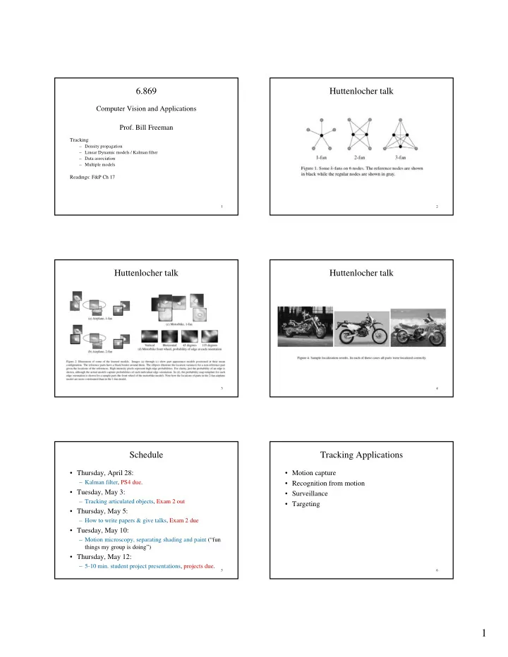
Huttenlocher talk
3
Huttenlocher talk
4
Huttenlocher talk
5
Schedule
- Thursday, April 28:
– Kalman filter, PS4 due.
- Tuesday, May 3:
– Tracking articulated objects, Exam 2 out
- Thursday, May 5:
– How to write papers & give talks, Exam 2 due
- Tuesday, May 10:
– Motion microscopy, separating shading and paint (“fun things my group is doing”)
- Thursday, May 12:
– 5-10 min. student project presentations, projects due.
6
- Motion capture
- Recognition from motion
- Surveillance
- Targeting