
SLIDE 1
1
Differential gene expression General Introduction
Swiss Institute of Bioinformatics - LF 11.2010
Swiss Institute of Bioinformatics - LF 11.2010Overview (1)
n
Reminder of biology
n
Major steps in microarray analysis
¡
Microarray preparation design, clone/probe selection
¡
RNA extraction, hybridization on chip
¡
Scanning, data extraction from image
¡
“Low-level” Quality Control
¡
Summarization of per-chip information (one number per feature)
¡
“High-level” analysis
n
High-throughput RNA-level technologies
¡
Microarrays
¡
Affymetrix Chips
¡
SAGE
¡
MPSS
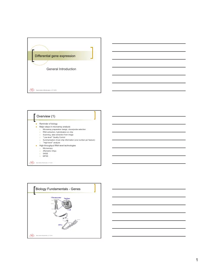
Swiss Institute of Bioinformatics - LF 11.2010Biology Fundamentals - Genes