1
play

1 Identical by descent (IBD): genes that originated by replication - PDF document

Population Genetics 3: Inbreeding Inbreeding: the preferential mating of closely related individuals Consider a finite population of diploids: What size is needed for every individual to have a separate ancestor ? every individual must have 2


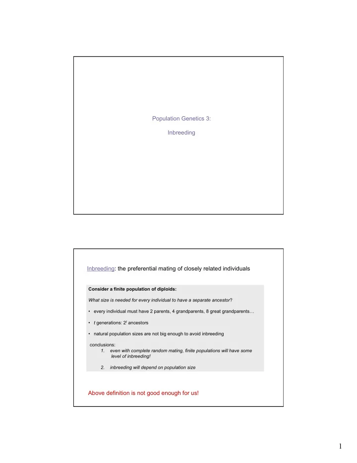
  1. Population Genetics 3: Inbreeding Inbreeding: the preferential mating of closely related individuals Consider a finite population of diploids: What size is needed for every individual to have a separate ancestor ? • every individual must have 2 parents, 4 grandparents, 8 great grandparents … • t generations: 2 t ancestors • natural population sizes are not big enough to avoid inbreeding conclusions: 1. even with complete random mating, finite populations will have some level of inbreeding! 2. inbreeding will depend on population size Above definition is not good enough for us! 1

  2. Identical by descent (IBD): genes that originated by replication of a single gene in a previous generation. Coefficient of inbreeding (F): the probability that any two alleles at a randomly chosen locus within a single individual are IBD. Inbreeding: 1. Individual inbreeding in a pedigree sense 2. Inbreeding as a population deviation from HWE 3. Inbreeding arising from a finite population size 2

  3. I. Individual inbreeding in a pedigree sense I. Individual inbreeding in a pedigree sense : Conventional pedigree Aa a a Males a a Females aa IBD First cousin mating 3

  4. I. Individual inbreeding in a pedigree sense : Inbreeding coefficient for individual 1 ( F 1 ) via “ path analysis ” : 1. Find each path that alleles might take to become IBD. 2. Count the number of lines ( n ) in each path (path segments). 3. Compute the probability of the path. 4. Sum the probabilities over all possible paths NOTE: F CA is the inbreeding coefficient of the common ancestor (CA) I. Individual inbreeding in a pedigree sense : Path 1: “ A ” is the CA Path 2: “ B ” is the CA Conventional representation Conventional representation Path 1 Path 1 Path 2 Path 2 A A B B A A A B B B Step 1: C C D D C C C C C C D D D D D D E E F F E E E F F F E E E F F F I I I I I I I I What is the inbreeding Step 2: coefficient for individual “ I ” ? Path 1: 6 segments Path 2: 6 segments 4

  5. A note about the common ancestor (CA) Path 1 Path 2 A B C C D D E F E F Source 2: It is also possible that X 1 and X 2 are IBD I I x 1 & x 2 = 1/4 x 2 & x 1 = 1/4 Segment 1 Segment 2 Probability x 1 x 1 ½ × ½ = ¼ x 1 x 2 ¼ ( ¼ ) F CA + ( ¼ ) F CA = ( ½ ) F CA x 2 x 1 ¼ x 2 x 2 ¼ Source 1 for IBD: same allele passed down both segments ( )  1 2 1 2 F +      CA Genotypes: X 1 X 1 or X 2 X 2 prob. that CA prob that CA transmited identical transmitte d diff ¼ + ¼ = ½ allele down both paths alleles that were IBD I. Individual inbreeding in a pedigree sense : Step 3: Compute the probability of the path (in our case 2 paths, each with n = 6 segments). Path 1 Probability of a path: Path 2 A B n 2 ( 1 2 ) − ( 1 2 ( 1 2 ) F ) × +    C       CA  D C D Probabilit y for n - 2 Probabilit y for two CA segments not connected segments; i.e., from last slide E F E F to CA I I n 2 ( ) − ( )( ) 1 / 2 1 2 1 F × + CA − 1 n 1 ( ) ( ) 1 / 2 F i + CA 5

  6. I. Individual inbreeding in a pedigree sense : Step 4 : Sum over all possible paths for IBD in pedigree Path 1 Path 2 − 1 A B n 1 F ( 1 / 2 ) ( F ) i = ∑ + 1 CA i C C D D E F E F paths in pedigree are indexed by i I I I. Inbreeding arising from a finite population size: Example: first cousin mating Conventional representation A B Case 1: Outbred ancestors F CA = 0 C D F I = (1/2) 6-1 (1+0) + (1/2) 6-1 (1+0) = 0.062 E F I Case 2: Inbred ancestors − 1 n 1 F ( 1 / 2 ) ( F ) i = ∑ + I CA F CA = 0.375 i F I = (1/2) 6-1 (1+0.375) + (1/2) 6-1 (1+0.375) = 0.09 i = 2 paths n = 6 segments 6

  7. II. Inbreeding as a population deviation from HWE II. Inbreeding as a population deviation from HWE: Now let ’ s consider the affect of inbreeding on HWE • let F = probability of IBD beyond random mating expectations. • let p = frequency of the A allele f AA = p 2 HWE: ⎡ ⎤ ⎢ ⎥ f AA p p ( 1 F ) F Inbreeding: = ⎢ − + ⎥        ⎢ ⎥ The prob of A The prob that The prob of A by mating with the first allele ⎢ ⎥ by random mating ⎣ a relative ⎦ was an A 7

  8. II. Inbreeding as a population deviation from HWE: Male gametes A (freq = p ) a (freq = q ) female gametes A AA Aa ( p ) p [ p (1- F ) + F ] p [ q (1- F )] a Aa aa ( q ) q [ p (1- F )] q [ q (1- F ) + F ] F inbreeding fraction of population (1- F ) random mating fraction of population II. Inbreeding as a population deviation from HWE: For AA, the frequency is: p[p(1- F ) + F ] p 2 + pqF AA = p[p - p F + F ] Aa = 2 pq (1 - F ) p 2 – p2 F + p F q 2 + pqF aa = p 2 + p F (1 – p) What does this tell us about genotype p 2 + pq F frequencies under inbreeding? 8

  9. II. Inbreeding as a population deviation from HWE: Genotype frequencies under inbreeding p 2 + pqF AA = Aa = 2 pq (1 - F ) By the way, remember this q 2 + pqF formula! aa = Example : A = p = 0.6, and a = q = 0.4 F = 0 (HW) F = 0.5 F = 1 AA = 0.36 AA = 0.48 AA = 0.6 [= p ] Aa = 0.48 Aa = 0.24 Aa = 0 aa = 0.16 aa = 0.28 aa = 0.4 [= q ] F = 0 is HWE F > 0 leads to a deficiency in heterozygotes (excess of homozygotes) F = 1 leads to a completely homozygous population II. Inbreeding as a population deviation from HWE: 1. Inbreeding yields change in the genotype frequencies of the population, but does not alter the allele frequencies. 2. Hence “losing variation to inbreeding” is only a loss of heterozygosity; there is no loss of allelic variation! 3. Inbreeding affects all loci in a genome. 4. Inbreeding slows the approach to equilibrium among loci; i.e., the decay of LD 9

  10. II. Inbreeding as a population deviation from HWE: Hierarchical F statistics: F = fractional reduction heterozygosity due to non-random mating F = (H HW – H)/H HW H = H HW – (H HW x F ) OK, that checks out Remember that H HW = 2 pq H = 2 pq – 2 pqF H = 2 pq (1 – F ) F ST = reduction of heterozygosity due to structure (non-random mating) within a population. Also called the fixation index. F ST = (H T – H S )/H T H T = The expected heterozygosity of an individual in a total population that is random mating H S = The expected heterozygosity of an individual in a subpopulation that is random mating III. Inbreeding arising from a finite population size 10

  11. III. Inbreeding arising from a finite population size: Let ’ s set up an idealized population with the following characteristics: 1. A finite population with N individuals 2. Each individual produced equal numbers of sperms and eggs 3. Sperm and eggs unite at random Let ’ s start out (generation = 0) with completely out-bred population: 1 The probability of randomly picking ones own allele F 0 = from the gamete pool is its frequency in the gamete 2 N pool III. Inbreeding arising from a finite population size: Let ’ s consider a second generation (generation = 1): 1 1 ⎛ − ⎞ F 1 F = + ⎜ ⎟ 1 0 2 N 2 N  ⎝ ⎠      prob of IBD prob of IBD by sampling ones from inbreeding in own gamete in previous generation s current generation We can extend this any number of generations (generation = g ): 11

  12. III. Inbreeding arising from a finite population size: 1 1 ⎛ − ⎞ F 1 F = + ⎜ ⎟ g g 1 − 2 N 2 N ⎝ ⎠ 1 F Δ = There is an incremental increase in 2 N inbreeding due to finite population size. We can think of this as “ the rate at which inbreeding accumulates ” . III. Inbreeding arising from a finite population size: We have a problem: • idealized populations do NOT exist! • natural populations will not behave according to the above formulas! • real populations have high variance in reproduction Inbreeding effective size ( N e ): the number of an otherwise ideal population which accumulates inbreeding effects at the same rate as the actual (non-ideal) population. 1 F Δ = 2 N e 12

  13. III. Inbreeding arising from a finite population size: Any factor that affects the variance in reproductive success will impact the N e Some important cases: 1. Fluctuating population sizes in successive generations 2. Different numbers of males and females 3. Variance in reproductive success (other than male verse female) III. Inbreeding arising from a finite population size: 1. Unequal numbers in successive generations 1 1 ⎡ 1 1 1 1 ⎤ ... (approx.) = + + + + ⎢ ⎥ N g N N N N ⎢ ⎥ e ⎣ 1 2 3 g ⎦ Harmonic mean because of the “ residual ” effect of historical levels of inbreeding • sensitive to bottleneck effect • census size could be very different from effective size Droughts, floods, etc. are examples of stochastic events that ensure the variance in N will be high over time 13

  14. III. Inbreeding arising from a finite population size: Effective population size is dominated by historical lows and can be very much lower than current census size. 120,000 Population crash population census size Population recovered to historical high 100,000 80,000 60,000 Ave N 40,000 20,000 N e 0 1 2 3 4 5 6 7 8 9 10 11 12 13 14 15 16 17 18 19 20 21 22 23 24 Time III. Inbreeding arising from a finite population size: 1. Very high variance in reproductive success among individuals 2. Very high variance in reproductive success among successive generations 14

Download Presentation
Download Policy: The content available on the website is offered to you 'AS IS' for your personal information and use only. It cannot be commercialized, licensed, or distributed on other websites without prior consent from the author. To download a presentation, simply click this link. If you encounter any difficulties during the download process, it's possible that the publisher has removed the file from their server.

Recommend


More recommend