[PDF] - 1 Multi-Slice CT Multi-Slice CT Wider beam widths Thinner PDF Document

SLIDE 1

1

IAEA Nov 06

S. Edyvean

Imaging Performance Assessment

f CT Scanners
St. Georges Hospital

www.impactscan.org

The impact of MDCT on optimisation and quality assurance of CT scanners

ImPACT ImPACT

IAEA Nov 06

2

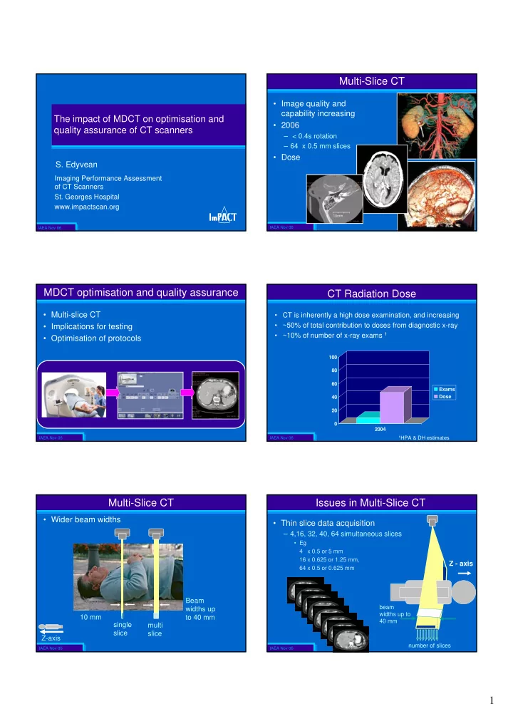
Multi-Slice CT

Image quality and

capability increasing

2006

– < 0.4s rotation – 64 x 0.5 mm slices

Dose

10mm

IAEA Nov 06

3

MDCT optimisation and quality assurance

Multi-slice CT
Implications for testing
Optimisation of protocols

IAEA Nov 06

4

CT Radiation Dose

CT is inherently a high dose examination, and increasing
~50% of total contribution to doses from diagnostic x-ray
~10% of number of x-ray exams 1

20 40 60 80 100 2004 Exams Dose

1HPA & DH estimates

IAEA Nov 06

6

Multi-Slice CT

single slice Z-axis Beam widths up to 40 mm 10 mm multi slice

Wider beam widths

IAEA Nov 06

7

Thin slice data acquisition

– 4,16, 32, 40, 64 simultaneous slices

Eg

4 x 0.5 or 5 mm 16 x 0.625 or 1.25 mm, 64 x 0.5 or 0.625 mm

Z - axis

Issues in Multi-Slice CT

beam widths up to 40 mm number of slices

SLIDE 2

2

IAEA Nov 06

8

10 mm 20, 24, 32 mm 29, 32, 40 mm

Multi-Slice CT

single slice 4 - 16 slice 64 slice

z-axis

Wider beam widths

IAEA Nov 06

9

Detector mock-ups courtesy of Toshiba 4 x 0.5 = 2 mm 16 x 0.5 = 8 mm 64 x 0.5 = 32 mm

Toshiba Aquilion series Z - axis

Multi-Slice CT

Thinner slices and more of them

IAEA Nov 06

10

Rotating tube and detectors – same as single slice
Many axial images
Helical scanning – many data sets

Power Data

20 mm

Multi-Slice CT

IAEA Nov 06

11

Axial scans

– Limited to ~ 16 slices, even on a 64 slice scanner – Cone beam effect

Multi-Slice CT

IAEA Nov 06

12

Recon position 1

Multi-Slice CT

Helical scanning – one acquisition

– All channels acquire data (4,16, 64 slice scanner) – Each image uses data from many detectors

IAEA Nov 06

13

Recon position 1

Multi-Slice CT

Helical scanning – one acquisition

– All channels acquire data (4,16, 64 slice scanner) – Each image uses data from many detectors – Reconstruct many images from one scan

SLIDE 3

3

IAEA Nov 06

14

Recon position 2

Multi-Slice CT

Helical scanning – one acquisition

– All channels acquire data (4,16, 64 slice scanner) – Each image uses data from many detectors – Reconstruct many images from one scan – Reconstruct other thicknesses – Most scanning done helically

IAEA Nov 06

15

Automatic exposure control

– Varying attenuation of, along, and around patients – Tube current automatically adjusted to achieve a standard noise level

Multi-Slice CT

From patient to patient Along patient length Around the patient

IAEA Nov 06

16

Multi-Slice CT

From patient to patient Along patient length Around the patient

Automatic exposure control

– Varying attenuation of, along, and around patients – Tube current automatically adjusted to achieve a standard noise level – Scanners do all or some

mA angle

180

+180

Low mA High mA mA

IAEA Nov 06

17

CT scanner technical quality

Purchase Acceptance Quality control

Quality control part of overall testing process
Many of the tests are the same

IAEA Nov 06

18

IAEA Nov 06

19

References and resources

www.ipem.org.uk www.impactscan.org

Part III Computed Tomography

IPEM Report 91 (2005) Chapter 12 CT IPEM Report 32 (2003) What to do and when How and why (IPEM) Institute of Physics and Engineering in Medicine

SLIDE 4

4

IAEA Nov 06

20

American College of Radiology www.acr.org

– CT Accreditation program (Med. Phys, 31 (9) September 2004) – Practical tips, artefact examples, pitfalls to avoid

AAPM, RSNA

– www.aapm.org – www.rsna.org

References and resources

IAEA Nov 06

21

Issues in multi-slice CT testing

Wider irradiated beam

– Is the test object long enough ?

Many slices acquired simultaneously

– Should I measure all the axial slices ? – Can I deal with all the images ?

Thinner slices

– Is the test object good enough ?

Automatic exposure control

– What should I do ?

Mainly helical protocols

IAEA Nov 06

22

CT scanner tests

Image quality

– image noise – imaged slice thickness – spatial resolution

Dose

– CTDI (in air, in phantom)

AEC

IAEA Nov 06

23

Image noise

noise image

Axial or helical scan
Noise = standard deviation (σ) of CT number in roi
roi ~ 40% of phantom diameter for repeatable results

region of interest (roi)

water filled phantom

IAEA Nov 06

24

Phantom long enough to accommodate all slices
Don’t forget scatter

Is the test object long enough ?

20 – 40 mm

ImPACT (30 → 120 mm) Catphan (20 → 40 mm) Manufacturer’s phantom

120

IAEA Nov 06

25

Should I measure all the axial slices ?

For equal noise in each slice need

– Equal sensitivity of detectors – Equal dose to detectors

On four slice scanners, outer slices ~ 5% higher

SLIDE 5

5

IAEA Nov 06

26

Should I measure all the axial slices ?

For equal noise in each slice need

– Equal sensitivity of detectors – Equal dose to detectors

On four slice scanners, outer slices ~ 5% higher

IAEA Nov 06

27

Measure all or some of the slices

Noise measurements in multi-slice

0.80 1.20 1.60

1 2 3 4 5 6 7 8 9 10 11 12 13 14 15 16

Slice # noise % Std Head Std Body

16 x 0.63 mm slices

IAEA Nov 06

28

All detectors contribute to image

– no need for four, eight or sixteen sets of images

Phantom length

– Need to account for extra rotations at either end – Don’t forget scatter

Noise measurements in multi-slice - helical

IAEA Nov 06

29

In axial scan - determined by detector group

Image slice thickness

fwhm

IAEA Nov 06

30

In helical scanning - interpolated from helical data

Image slice thickness

fwhm

IAEA Nov 06

31

A typical test object – aluminium inclined plate
Some use wire, at 25, 30, or 45 º
0.6 mm Al plate,
30 degrees to scan plane

z-axis

Image slice thickness - axial

SLIDE 6

6

IAEA Nov 06

32

Shown by width of plate projected into image
Corrected for angle of plate

z-axis

Test object Imaged slice

Image slice thickness - axial

fwhm

IAEA Nov 06

33

Most inserts are not long enough to measure all slices
Scan in two positions

Multi-slice imaged slice width - axial

z-axis

16 slices

IAEA Nov 06

34

Beware slice at end of inclined plate

– Image may look roughly ok, but data not true

Note end slice – cone beam effect

Multi-slice imaged slice width - axial

z-axis

16 slices fwhm Slice at end of plate

IAEA Nov 06

35

As number of slices increases, beam is more

diverging, outer slices are distorted single four sixteen

Multi-Slice CT

IAEA Nov 06

36

central slice

uter slice (16 slice)

Multi-slice imaged slice width - axial

IAEA Nov 06

37

Multi-slice imaged slice width - axial

0.48 0.5 0.52 0.54 0.56 0.58 0.6 0.62

1 2 3 4 5 6 7 8 9 10 11 12 13 14 15 16

Slice number fwhm (mm)

Measure all or some of the slices

SLIDE 7

7

IAEA Nov 06

38

Measurement of slice widths of < 1mm

– not possible where thickness of plate is < or = image width

ImPACT use two phantoms

– 0.5 mm aluminium, 30° (slices 2 - 20 mm) – 0.05 mm titanium, 8° (slices 0.5 - 4 mm)

Is my test object good enough ?

IAEA Nov 06

39

z-axis

Shallow angle gives more pixels in projection in image
More plates extend phantom in z-direction whilst staying

close to the centre of the field of view

Multi-slice imaged slice width - axial

8°

pixel values

IAEA Nov 06

40

High contrast bead or disc
Same test for single and multi-slice

perspex rod tungsten disk 0.05 mm

Imaged slice width – helical

IAEA Nov 06

41

50 100 150 200

10
8
6
4
2

2 4 6 8 10

mm CT Numbers

2.5mm 5mm

FWTM FWHM

Scan test object

– Images reconstructed at sub-slice intervals – CT number in each image used to create the profile

Imaged slice width – helical

perspex rod

Helical Z-Sensitivity tool

0.05 mm tungsten thin disk

IAEA Nov 06

42

Scan plane spatial resolution

Subjective

– visual assessment of repeating pattern

Objective

– calculation of MTF

edge
bead, wire

10 20 30 40 50 60 70 80 90 100 2 4 6 8 10 Frequency (lp/cm) MTF (%)

IAEA Nov 06

43

Same test for single and multi-slice
Use for both axial and helical images
Only need measure for one axial image

– Factors affecting scan plane spatial resolution are in the scan plane, and do not change from slice to slice

MSCT - Scan plane spatial resolution

SLIDE 8

8

IAEA Nov 06

44

Dose

Computed tomography dose index (CTDI)
Measured with 100 mm ion chamber

– In air for quality control – In phantom for acceptance, dose reference levels

IAEA Nov 06

45

CTDI on multi-slice scanners

Use total nominal beam width (n.T)

ion chamber Z-axis Eg n.T = 4 x 2.5 mm = 10 mm

CTDI = dose x chamber length (n.T)

n = no. slices imaged simultaneously T = nominal imaged width n.T = total detection width = nominal beam width

∫

+ −

=

50 50

D(z)dz n.T 1 CTDI100

IAEA Nov 06

46

More scatter, but proportionally the same
As a dose index, CTDI ok for larger beam widths

air centre phantom

What about wider beam widths ?

IAEA Nov 06

47

Testing the AEC

Test object needs to vary in z-direction and rotationally

– eg Conical Perspex phantom with elliptical cross section End view Side view

CT scanner couch Catphan carrying case

Based on ‘Apollo’ phantom developed by

Muramatsu, National Cancer Centre, Tokyo

IAEA Nov 06

48

Images along length of phantom (no AEC)

Constant mA

Testing the AEC

IAEA Nov 06

49

Testing the AEC

Measure noise with AEC off and on
Monitor mA, CTDIvol

GE LightSpeed16

4 8 12 16 20 24 28

150
100
50

50 100 150 Z-position (mm) Noise (%) automA off Noise Index 12

Increased mA Decreased mA

www.impactscan.org/bluecover.htm

Constant mA

Same mA Increased mA Decreased mA

SLIDE 9

9

IAEA Nov 06

50

Coronal view Sagittal view z-axis AEC off z-axis AEC on

Noise increases Constant noise

Testing the AEC – Viewing with MPR

IAEA Nov 06

Circular, elliptical phantoms of various sizes
Scan short lengths over each section
Monitor mA, CTDIvol, image noise

Testing the AEC

IAEA Nov 06

52

Which scan protocols ?

Nominal image width ^^ ^^ ^^ Pitch ^

Scan plane resolution

Interpolation algorithm Convolution kernel Detector group size * Beam width Scan time Focal spot selection kV mA

Dose Image width Noise

^ If scan time affects no. samples, ^^ In some circumstances , * In almost all cases

IAEA Nov 06

53

Time constraints of quality control

– Use typically used protocols – Many are helical, axial gives good basic data

Rotate through to ensure all modes are looked at

Courtesy Elly Castallano, Royal Marsden Hospital, London

2 sec scan

Which scan protocols ?

IAEA Nov 06

54

Courtesy Elly Castallano, Royal Marsden Hospital, London

Which scan protocols ?

2 sec scan

IAEA Nov 06

55

Large amount of data

– Think through the testing carefully – Can you handle the data you are generating ? – Do you need to consider an automated process ?

Testing of multi-slice scanners

SLIDE 10

10

IAEA Nov 06

56

Data analysis

Analysis tools, need programming

– IDL, MatLab, C# – UK CT Users Group,16 Nov 2006 (ctug.org.uk) looking at this issue

IAEA Nov 06

57

Multi-slice CT
Implications for testing
Optimisation of protocols

Penumbra typically 3 mm for all beam widths

– lower proportion of total dose with larger beam widths

Wider is generally better

z-axis 8 slice 4 slice 16 slice GE LightSpeed: 4, 8, 16 - slice 10 mm (8 x 1.25) 20 mm (16 x 1.25) 5 mm (4 x 1.25) Collimation 17 3 33 Penumbra dose (%)

IAEA Nov 06

61

Beam width

To image entire volume, extra rotations are needed

at both ends of scan

– This is larger for wide beam widths

Significant when using short scan lengths, or higher

pitches

64

Thinner slice: improved contrast

Better contrast for small structures

Wide slice Narrow slice – same mAs

IAEA Nov 06

Automatic exposure control

Most systems allow users to set a required noise level

– An image noise index – Specifying a reference image with acceptable image quality

Maximum and minimum mA sometimes specified

Eg GE Auto mA

IAEA Nov 06

66

Smart mA – LightSpeed Pro 16

100 mA 170 mA

Automatic exposure control

GE Auto mA

– Varies mA along patient 210 mA 220 mA

Courtesy: GE Medical / Eugenia Kulama Royal Marsden Hospital London IAEA Nov 06

67

Automatic exposure control

Additional benefit

– Reduction of artefacts with rotational AEC – Low photon count in lateral projections gives streak artefacts

Courtesy: Siemens / Eugenia Kulama Royal Marsden Hospital London

171 mAs Scan with real-time dose modulation 327 mAs Scan with constant mA

Siemens CAREDOSE (4D)

SLIDE 12

12

IAEA Nov 06

68

What do AECs give us?

Lower patient doses than before?

– Possibly, but not necessarily – It is possible to use AEC and give higher dose

‘dose can go up as well as down’
More consistent image quality?

– Yes

The optimum image quality?

– If they are used well

What is the required image noise?

Dose Ratio: 0.83 SD: 8.5

IAEA Nov 06

72

Simulation

Plain Early Late

Images courtesy Y. Muramatsu, NCC Tokyo

What noise level is needed?

Dose Ratio: 0.67 SD: 9.0

IAEA Nov 06

73

Simulation

Plain Early Late

Images courtesy Y. Muramatsu, NCC Tokyo

What noise level is needed?

Dose Ratio: 0.50 SD: 10.0

What noise level is needed?

Dose Ratio: 0.04 SD: 42.0

SLIDE 14

14

IAEA Nov 06

80

MDCT optimisation and quality assurance

Multi-slice CT
Implications for testing
Optimisation of protocols

IAEA Nov 06

S. Edyvean

Imaging Performance Assessment

f CT Scanners
St. Georges Hospital