1 Evolution events of CP 1970s: Image processing applications in - - PDF document

1

ACP Summer School on Theory and Practice of Constraint Programming September 24-28, 2012, Wrocław, Poland Willem-Jan van Hoeve Tepper School of Business, Carnegie Mellon University

Introduction to Constraint Programming Outline

General introduction

• Successful applications
• Modeling
• Solving
• CP software

Basic concepts

• Search
• Constraint propagation
• Complexity

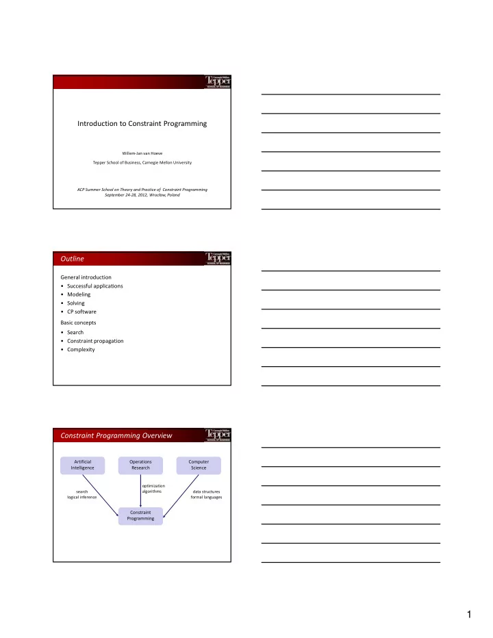
Constraint Programming Overview

Constraint Programming Artificial Intelligence Operations Research Computer Science

search logical inference

• ptimization

algorithms data structures formal languages

2

Evolution events of CP

1980s: Logic Programming (Prolog); Search + logical inference 1970s: Image processing applications in AI; Search+qualitative inference 1990s: Constraint Programming; Industrial Solvers (ILOG, Eclipse,…) 2000s: Global constraints; integrated methods; modeling languages 1994: Advanced inference for alldifferent and resource scheduling 1989: CHIP System; Constraint Logic Programming 2006: CISCO Systems acquires Eclipse CLP solver 2009: IBM acquires ILOG CP Solver & Cplex

Successful applications Sport Scheduling

Schedule of 1997/1998 ACC basketball league (9 teams)

• various complicated side constraints
• all 179 solutions were found in 24h using enumeration and integer

linear programming [Nemhauser & Trick, 1998]

• all 179 solutions were found in less than a minute using constraint

programming [Henz, 1999, 2001]

Week 1 Week 2 Week 3 Week 4 Week 5 Week 6 Week 7 Period 1 0 vs 1 0 vs 2 4 vs 7 3 vs 6 3 vs 7 1 vs 5 2 vs 4 Period 2 2 vs 3 1 vs 7 0 vs 3 5 vs 7 1 vs 4 0 vs 6 5 vs 6 Period 3 4 vs 5 3 vs 5 1 vs 6 0 vs 4 2 vs 6 2 vs 7 0 vs 7 Period 4 6 vs 7 4 vs 6 2 vs 5 1 vs 2 0 vs 5 3 vs 4 1 vs 3

3

Hong Kong Airport

• Gate allocation at the Hong Kong International Airport
• System was implemented in only four months, and includes

constraint programming technology (ILOG)

• Schedules ~900 flights a day (53 million passengers in 2011)

8

Port of Singapore

• One of the world’s largest container transshipment hubs
• Links shippers to a network of 200 shipping lines with connections to

600 ports in 123 countries

• Problem: Assign yard locations and loading plans under various
• perational and safety requirements
• Solution: Yard planning system, based on constraint programming

(ILOG)

Railroad Optimization

• Netherlands Railways has among the densest rail networks in

the world, with 5,500 trains per day

• Constraint programming is one of the components in their

railway planning software, which was used to design a new timetable from scratch (2009)

• Much more robust and effective schedule, and $75M additional

annual profit

• INFORMS Edelman Award winner (2009)

4

CP Modeling and Solving

• CP allows a very flexible modeling language
• Virtually any expression over the variables is allowed

e.g., x3(y2 – z) ≥ 25 + x2∙max(x,y,z)

• CP models can be much more intuitive than, e.g., MIP
• r SAT models

close to natural language

10

CP Variables

• CP variable types include the classical:

binary, integer, continuous

• In addition, variables may take a value from any

finite set

e.g., x in {a,b,c,d,e} the set of possible values is called the domain of a variable

• Lastly, there exist special `structured’ variable types

set variables (take a set of elements as value) activities or interval variables (for scheduling applications)

11

CP Constraints – Examples

• Algebraic expressions:

x3(y2 – z) ≥ 25 + x2∙max(x,y,z)

• Extensional constraints (‘table’ constraints):

(x,y,z) in MyTupleSet

• Variables as subscripts (‘element’ constraints):

y = cost[x] (here y and x are variables, ‘cost’ is an array of parameters)

• Reasoning with meta-constraints:

∑i (xi > Ti) ≤ 5

• Logical relations in which (meta-)constraints can be mixed:

((x < y) OR (y < z)) (c = min(x,y))

• Global constraints:

Alldifferent(x1,x2, ...,xn) DisjunctiveResource( [start1,..., startn], [dur1,...,durn], [end1,...,endn] )

5

CP vs MIP Modeling: Task Sequencing

• We need to sequence a set of tasks on a machine

Each task i has a specific fixed processing time pi Each task can be started after its release date ri, and must be completed before its deadline di Tasks cannot overlap in time

Time is represented as a discrete set of time points, say {1, 2,…, H} (H stands for horizon)

13

MIP model

• Variables

Binary variable xij represents whether task i starts at time period j

• Constraints

Each task starts on exactly one time point ∑j xij = 1 for all tasks i Respect release date and deadline j*xij = 0 for all tasks i and (j < ri) or (j > di - pi)

14

MIP model (cont’d)

• Tasks cannot overlap

variant 1 ∑i xij ≤ 1 for all time points j we also need to take processing times into account; this becomes messy variant 2 introduce binary variable bik representing whether task i comes before task k must be linked to xij; this becomes messy

15

6

CP model

• Variables

Let starti represent the starting time of task i takes a value from domain {1,2,…, H} This immediately ensures that each task starts at exactly one time point

• Constraints

Respect release date and deadline ri ≤ starti ≤ di - pi

16

CP model

• Tasks cannot overlap:

for all tasks i and j

(starti + pi < startj) OR (startj + pj < starti) That’s it! (See also Lombardi’s lectures on scheduling for more advanced models)

17

Benefits of CP model

• The number of CP variables is equal to the number of

tasks, while the number of MIP variables depends also

• n the time granularity (for a horizon H, and n tasks,

we have H*n binary variables xij)

• The sequencing constraints are quite messy in MIP,

but straightforward and intuitive in CP

18

7

Variables as subscripts: the TSP

• The traveling salesperson problem asks to find a

closed tour on a given set of n locations, with minimum total length

• Input: set of locations and distance dij between two

locations i and j

19

• Classical model based on ‘assignment problem’ 1
• Binary variable xij represents whether the tour goes

from i to j

• Objective

min ∑ij dijxij

1 Alternative MIP models exist, for example the time-indexed

formulation uses yijt = 1 if we traverse (i,j) at step t

TSP: MIP model

20

3 2 4 5 6 1

• Need to make sure that we leave and enter

each location exactly once

∑j xij = 1 for all i ∑i xij = 1 for all j

• Constraints to remove all possible

subtours:

there are exponentially many

MIP methodology therefore applies specialized solving methods for the TSP

3 2 4 5 6 1 3 2 4 5 6 1

TSP: MIP model (cont’d)

21

8

TSP: CP model

• Variable xi represents the i-th location that the tour

visits (variable domain is {1,2,…,n} )

• Objective

min

• Constraint

alldifferent(x1, x2, …, xn)

22

dxn ,x1 + dxi ,xi+1

i=1 n−1

• ‘global’ constraint

variables can be used as subscripts!

MIP and CP model compared

• The CP model needs only n variables, while the MIP

model needs n2 variables (n is #locations)

• The MIP model is of exponential size, while the CP

model only needs one single constraint (and element contraints)

• The CP model is perhaps more intuitive, as it is based

directly on the problem structure: the ordering of the locations in the tour

Note: The specialized MIP solving methods outperform CP on pure

• TSP. In presence of side constraints (e.g., time windows), CP is
• ften much faster than MIP.

23

CP Solving

In general

• CP variables can be

discrete (i.e., integer valued)

• CP constraints can be

non-linear non-differentiable discontinuous

Hence, no traditional exact Operations Research technique (LP, NLP, MIP, etc) can solve these models

24

9

Basics of CP solving

• CP solving is based on intelligently enumerating all

possible variable-value combinations

backtracking search

• At each search state, CP applies specific constraint

propagation algorithms

• These propagation algorithms are applied to individual

constraints, and their role is to limit the size of the search tree

25

Example: Graph coloring

26

Assign a color to each country Adjacent countries must have different colors Can we do this with at most four colors?

Smaller (8 variable) instance

27

x1 x2 x3 x4 x5 x8 x6 x7

10

CP Model

28

x1 x2 x3 x4 x5 x8 x6 x7 x1 x2 x3 x4 x5 x8 x6 x7

Constraints: xi ≠ xj for all edges (i,j) Variables and domains: xi in {r,g,b,p} for all i

CP Solving

29

x1 x2 x3 x4 x5 x8 x6 x7 x1 x2 x3 x4 x5 x8 x6 x7

rgbp rgbp rgbp rgbp rgbp rgbp rgbp rgbp

Constraint propagation: can we remove inconsistent domain values?

Search

30

x1 x2 x3 x4 x5 x8 x6 x7 x1 x2 x3 x4 x5 x8 x6 x7

rgbp rgbp rgbp rgbp rgbp rgbp rgbp rgbp

Search: guess a value for a variable (but be prepared to backtrack): x2 = r

11

Propagate

31

x1 x2 x3 x4 x5 x8 x6 x7 x1 x2 x3 x4 x5 x8 x6 x7

rgbp rgbp rgbp rgbp rgbp r rgbp rgbp

Constraint propagation

Search

32

x1 x2 x3 x4 x5 x8 x6 x7 x1 x2 x3 x4 x5 x8 x6 x7

gbp gbp gbp rgbp rgbp r gbp gbp

Search: guess a value for a variable (but be prepared to backtrack): x5 = g

Propagate

33

x1 x2 x3 x4 x5 x8 x6 x7 x1 x2 x3 x4 x5 x8 x6 x7

gbp gbp g rgbp rgbp r gbp gbp

Constraint propagation

12

Search

34

x1 x2 x3 x4 x5 x8 x6 x7 x1 x2 x3 x4 x5 x8 x6 x7

gbp bp g rbp rbp r gbp bp

Search: guess a value for a variable (but be prepared to backtrack): x4 = b

Continuing search & propagate

35

x1 x2 x3 x4 x5 x8 x6 x7 x1 x2 x3 x4 x5 x8 x6 x7

gp b g rp rbp r gbp bp

Next search choice: x6 = b

Continuing search & propagate

36

x1 x2 x3 x4 x5 x8 x6 x7 x1 x2 x3 x4 x5 x8 x6 x7

gp b g rp rp r gp b

Next search choice: x8 = p

13

Continuing search & propagate

37

x1 x2 x3 x4 x5 x8 x6 x7 x1 x2 x3 x4 x5 x8 x6 x7

g b g p r r gp b

Next search choice: x3 = g

Continuing search & propagate

38

x1 x2 x3 x4 x5 x8 x6 x7 x1 x2 x3 x4 x5 x8 x6 x7

g b g p r r g b

We found a solution!

Solution

39

x1 x2 x3 x4 x5 x8 x6 x7 x1 x2 x3 x4 x5 x8 x6 x7

g b g p r r g b

14

CP Solving - Summary

The solution process of CP interleaves

• Domain filtering

remove inconsistent values from the domains of the variables, based on individual constraints

• Constraint propagation

propagate the filtered domains through the constraints, by re-evaluating them until there are no more changes in the domains

• Search

implicitly all possible variable-value combinations are enumerated, but the search tree is kept small due to the domain filtering and constraint propagation

Search tree for graph coloring example

41

x2 = r x2 ≠ r x5 = g x5 ≠ g x4 = b x4 ≠ b x6 = b x6 ≠ b x8 = b x8 ≠ b x3 = g x3 ≠ g

Observations

• depth-first search (DFS)

linear memory requirements applied in most CP systems

• search tree can be deep

considered 6 out of 8 variables depth ‘controls’ the exponential explosion of the search

How can we make the search tree smaller in general?

Can we color the graph with 3 colors?

42

x1 x2 x3 x4 x5 x8 x6 x7 x1 x2 x3 x4 x5 x8 x6 x7

rgb rgb rgb rgb rgb rgb rgb rgb

Search choice: x2 = r (by symmetry, no need to consider x2 = g, b)

x2 = r

15

Search & propagate

43

x1 x2 x3 x4 x5 x8 x6 x7 x1 x2 x3 x4 x5 x8 x6 x7

gb gb gb rgb rgb r gb gb

Search choice: x5 = g (be prepared to backtrack)

x2 = r x5 = g x5 ≠ g

Search & propagate

44

x1 x2 x3 x4 x5 x8 x6 x7 x1 x2 x3 x4 x5 x8 x6 x7

gb b g rb rb r gb b

… and propagate x7 has an empty domain: we need to backtrack

x2 = r x5 = g x5 ≠ g

Search & propagate

45

x1 x2 x3 x4 x5 x8 x6 x7 x1 x2 x3 x4 x5 x8 x6 x7

gb gb b rgb rgb r gb gb

Propagate…

x2 = r x5 = g x5 ≠ g

16

Search & propagate

46

x1 x2 x3 x4 x5 x8 x6 x7 x1 x2 x3 x4 x5 x8 x6 x7

gb g b rg rg r gb g

x2 = r x5 = g x5 ≠ g

Search & propagate

47

x1 x2 x3 x4 x5 x8 x6 x7 x1 x2 x3 x4 x5 x8 x6 x7

gb g b rg rg r gb g

…and propagate x7 has an empty domain: we are done

x2 = r x5 = g x5 ≠ g

Recall example: first propagation

48

x2 x3 x4 x5 x8 x6 x7 x1 x8

gb gb gb rgb rgb r gb gb

Can we do more propagation? After x2 = r we are done.

x2 = r

rgb rgb rgb rgb rgb

x3 x1 x5 x7 x6 x2 x4

17

Introduce global constraints

• We can increase the inference by adding more

knowledge to the solver

in this case, group not-equal constraints that form a clique use alldifferent constraints alldifferent(x1,x2,...,xn) := ∧i<j xi ≠ xj Model 1: x1 ∈ {g,b}, x4∈ {g,b}, x8∈ {r,g,b} x1 ≠ x4, x1 ≠ x8, x4 ≠ x8 Model 2: x1 ∈ {g,b}, x4∈ {g,b}, x8∈ {r,g,b} alldifferent(x1,x4,x8)

49

no propagation x8 = r x4 x8 x1 x8

gb gb rgb

x1 x4

Impact of global constraint propagation

• See graph.aimmspack
• Graph coloring problem; random instances
• Can set alldifferent propagation level from ‘low’ to

‘extended’

‘low’: pairwise not-equal constraints ‘extended’: best possible propagation notice the difference in search tree size (search choices or failures) and solving time

50

Global Constraints Summary

• Examples

Alldifferent, Count, BinPacking, SequentialSchedule, ParallelSchedule, NetworkFlow, …

• Global constraints represent combinatorial structure

can be viewed as the combination of elementary constraints expressive building blocks for modeling applications embed powerful algorithms from OR, Graph Theory, AI, CS, …

• Essential for the successful application of CP

When modeling a problem, always try to identify possible global constraints that can be used

18

Embedded Algorithms

Constraint Structure/technique alldifferent bipartite matching [Régin, 1994] cardinality network flow [Régin, 1999, 2002] knapsack dynamic programming [Trick, 2003] regular directed acyclic graph [Pesant, 2004] circuit network flow [Genc Kaya & Hooker, 2006] weighted circuit AP [Focacci et al, 1999], 1-Tree [Benchimol et al., 2012] sequence dedicated algorithm [vH et al., 2006, 2009] [Maher et al., 2009] disjunctive/cumulative dedicated algorithm [Nuijten 1994, Carlier et al., 1994] [Vilim, 2009] inter-distance dedicated algorithm [Quimper et al., 2006] . . .

. . .

The ‘global constraint catalog’ currently contains 354 constraints http://www.emn.fr/z-info/sdemasse/gccat/

Constraint Programming Solvers

Commercial

• IBM ILOG CP Optimizer

C++ library; free for academic users

• Kalis (Artelys / Fico)

C++ library

• SICSTUS-Prolog

Prolog-based library

• CHIP V5 (Cosytec)

C++/Prolog-based library

• Comet (Dynadec)

C++ library; free for academic users

• SCIP 1

C library; free for academic users

1 SCIP actually solves ‘constraint integer programs’ and combines MIP/LP

solving with CP and SAT techniques

Constraint Programming Solvers (cont’d)

Non-commercial (in terms of licensing)

• Gecode

C++ library

• Eclipse

Prolog-based library

• Google OR-tools

C++ library

• Choco

Java library

• JaCoP

Java library

• Minion

black-box solver; specific problem input

• Mistral

C++ library

19

CP Modeling Systems

Commercial

• IBM ILOG OPL

CP Optimizer, CPLEX (LP/MIP/QP)

• Xpress Mosel

Kalis, Xpress (LP/MIP/QP/NLP)

• AIMMS

CP Optimizer, most commercial LP/MIP solvers, and NLP solvers

• Comet

Comet, lp_solve, SCIP

Non-commercial / Academic

• Zinc, MiniZinc (G12)

Gecode, JaCoP

• Numberjack (python)

Mistral, SCIP

• Tailor/Essence

Minion

55

Hands-on Session

• Tomorrow (Tuesday) there will be a hands-on session

application: vehicle routing with side constraints integrated model: LP-based column generation with CP scheduling model

• We will use the AIMMS software for this

you can also use your favorite other CP system, but make sure it can link to an LP solver and has CP scheduling functionality if you want to use AIMMS, please make sure to have it installed before the session starts (let me know if you have issues) there will also be PCs in the lab running AIMMS

56

Get started with AIMMS

• One-hour tutorial (general introduction)
• Extensive documentation on CP functionality in the

manuals under `help’

• Example CP models

sudoku graph coloring single machine scheduling see: http://www.andrew.cmu.edu/user/vanhoeve/summerschool

57

20

Outline

General introduction

• Successful applications
• Modeling
• Solving
• CP software

Basic concepts

• Search
• Constraint propagation
• Complexity

59

Constraint Satisfaction Problems

A Constraint Satisfaction Problem, or CSP, consists of

• set of variables ,
• variable domains (v) (v∈),
• and set of constraints on the variables.

A solution to a CSP:

assign to each variable a single element from its domain such that all constraints are satisfied.

A constraint solver has to

• find a solution to a CSP,
• or prove that no solution exists.

60

Example: Graph Coloring

Coloring the nodes of the graph: What is the minimum number of colors such that any two nodes connected by an edge have different colors?

21

61

Graph Coloring - Model

variables : A,B,C,D,E,F domains : {r,b,g,y,c,p} constraints : A≠B, A≠C, A≠E, A≠F, B≠C, B≠D, B≠F, C≠D, C≠E, D≠E, D≠F, E≠F

C A F B D E 62

Graph Coloring – Simple Solver

• C

A F B D E

• 63

Graph Coloring – Simple Solver

• C

A F B D E

22

64

Graph Coloring – Simple Solver

• C

A F B D E

• ! "#

⋅##

• 65

Graph Coloring – Constraint Solver

• C

A F B D E

• 66

Graph Coloring – Constraint Solver

• C

A F B D E

23

67

Graph Coloring – Constraint Solver

• C

A F B D E

• 68

Graph Coloring – Constraint Solver

• C

A F B D E

• 69

Graph Coloring – Constraint Solver

• C

A F B D E

24

70

Graph Coloring – Constraint Solver

• C

A F B D E

• 71

Graph Coloring – Constraint Solver

• C

A F B D E

• ! $%

72

Constraint Solver

A constraint solver interleaves

• search

and constraint propagation

→ &!'!&() → &!'!&()

exponential size in general reduce size of search tree

25

73

Search Tree

A search tree can be defined by

• enumeration

choose a variable v from choose an element e from (v) branch v=e versus v≠e

• partitioning

choose a variable v from choose a subset S of elements from (v) branch v∈S versus v∉S

• branching constraints

for example x≤y versus x>y

Solving process heavily dependent on variable (and value) selection heuristics

' ' '∈* '∉* +, +- 74

Propagation

Constraint propagation makes the domains consistent with each individual constraint: Definition: a constraint C is domain consistent if all elements of all variable domains belong to a solution to C.

• +

$#

• $#
• +.

not domain consistent

• +

$

• #
• +.

domain consistent also known as ‘arc consistent’

75

Propagation

Q: How can we make a constraint domain consistent? A: Reduce the domains of the variables in the constraint. Such a procedure is called a domain filtering algorithm or ‘propagation’ algorithm

26

76

Propagation

A basic propagation algorithm for a constraint C looks as follows: bool Propagate(C,C,) { for all v∈C { for all e∈(v) { find a solution to C with v=e; if no solution exists, remove e from (v); if (v) is empty return false; } } return true; }

• +

$#

• $#
• +.

77

Propagation

A CSP usually consists of several constraints. What about constraint interaction? Definition: A CSP is domain consistent if all its constraints are.

• +

#

• #

/

• ()

+0, () 1 (+/)

()

• +

#

• /
• ()
• +

#

• /
• ()
• +

#

• /
• ()
• +

#

• /
• 78

Propagation Cycle

More formally, a CSP is made domain consistent by a Propagation Cycle:

bool Propagation_Cycle(,, Q := ; while Q nonempty { pick v in ; Q := Q - v; for all constraints C in containing v { if (Propagate(C,C,) == false) return false; if a domain of variable x has changed, set Q := Q + x; } } return true; } Note: this process always reaches a fix-point (i.e. either domain consistency or a failure). Alternative: store active constraints in Q

27

79

Solving process

Search + Constraint Propagation:

... ... ... ... ... Propagation_Cycle Branch Propagation_Cycle Branch Propagation_Cycle Branch Propagation_Cycle Branch

80

Solving process

Search + Constraint Propagation:

bool Solve(,,){ if |(v)| == 1 for all v in { return true; // we found a solution! } else { if (Propagation_Cycle(,,) == false) { return false; } else { choose variable v in with |(v)| > 1; choose element e in (v); return ( Solve(,,‘v=e’) OR Solve(,,‘v≠e’) ); } } }

81

Complexity of propagation

Consider binary constraint x < y, given as a ‘table’:

• +

$

• #
• 2

$

• #
• 2
• Example:

+∈$# ∈$# +.

• +

$

• #

$

• #
• check all elements in D(x) for support

check all elements in D(y) for support this takes O(|(x)|⋅|(y)|) time. This is the general time complexity to make binary constraints domain consistent.

28

82

More efficient propagation

Consider binary constraint x < y again.

Example: x∈{0,1,2,3,4} y∈{0,1,2,3} x < y

Note that this constraint is domain consistent iff

min(x) < min(y) and max(x) < max(y)

So we can make the constraint domain consistent by:

remove from D(y) all values ≤ min(x) remove from D(x) all values ≥ max(y)

This takes O(1) time (update the bounds of the domains). Much more efficient than generic algorithm.

83

Complexity of propagation

What about non-binary constraints? Consider the n-dimensional ‘table’ for a constraint on n variables v1,v2,...,vn. To check all domain elements for support we may need to traverse the whole space (v1) × (v2) × ⋅ ⋅ ⋅ × (vn). Hence, in general it is intractable to make non-binary constraints domain consistent! Notorious Example: the constraint Σi=1..n ci⋅xi = b

(ci and b are integer constants, xi integer variables (i=1..n)).

84

Complexity of propagation

Fortunately, some non-binary constraints can be made domain consistent in polynomial time! Example: alldifferent(x1,x2,...,xn) A solution to this constraint has a special structure1, and there exists an efficient algorithm to find it.

1 See next lecture.

29

85

Bounds consistency

In many cases we do not know a special structure to exploit. We can sometimes handle those difficult non-binary constraints by relaxing the consistency. Instead of domain consistency, we demand for example bounds consistency. Definition: a constraint C is bounds consistent if the bounds of all variable domains belong to a solution to C, where all domains are treated as intervals [ min(D(x)), max(D(x)) ].

(Note: we assume that the domains are all drawn from a totally ordered ground set.)

Example: Σi=1..n ci⋅xi = b can be made bounds consistent in polynomial time.

86

Complexity of propagation

Theorem: If all constraints can be made consistent in poly-time, then the Propagation Cycle runs in poly-time. Proof:

bool Propagation_Cycle(,, Q := ; while Q nonempty { pick v in ; Q := Q - v; for all constraints C in containing v { if (Propagate(C,C,) = false) return false; if a domain of variable x has changed, set Q := Q + x; } } return true; }

In each loop, either |Q|:=|Q|-1, or some domain element is removed. So there are at most n+n⋅d loops (for n variables with maximum domain size d).

87

Boundary of Polynomial Complexity

Recall that we can model the graph coloring problem as variables : x1, x2, …, x8 domains : {r,b,g,p} constraints : alldifferent(K) for all cliques K in the graph. Domain consistency for alldifferent is poly-time, Propagation Cycle is poly-time, → graph coloring is poly-time? But as graph coloring is NP-hard, do we have P = NP? No, finding maximum clique is NP-hard!

x1 x2 x3 x4 x5 x8 x6 x7 x1 x2 x3 x4 x5 x8 x6 x7

30

88

Consistency: counterexample

Moreover, even if we have alldifferent constraints for all cliques, it is not sufficient to determine consistency of the CSP:

• #
• #

#

• #

# #

• all constraints on

single edges are domain consistent

89

Consistency: counterexample

• #
• #

#

• #

# #

• clique is domain consistent

Moreover, even if we have alldifferent constraints for all cliques, it is not sufficient to determine consistency of the CSP:

90

Consistency: counterexample

• #
• #

#

• #

# #

• clique is domain consistent

Moreover, even if we have alldifferent constraints for all cliques, it is not sufficient to determine consistency of the CSP:

31

91

Consistency: counterexample

• #
• #

#

• #

# #

• but there is no solution!

try

Moreover, even if we have alldifferent constraints for all cliques, it is not sufficient to determine consistency of the CSP:

92

Consistency: counterexample

• #
• #

#

• #

# #

• #

Moreover, even if we have alldifferent constraints for all cliques, it is not sufficient to determine consistency of the CSP:

but there is no solution! try

93

Consistency: counterexample

• #
• #

#

• #

# #

• #

but there is no solution! try

Moreover, even if we have alldifferent constraints for all cliques, it is not sufficient to determine consistency of the CSP:

32

94

Summary of Complexity of CSP Solving

Message: NP-hard problems remain NP-hard. However, with constraint programming we can control (to some extent) where to put the NP-hardness:

• exponential-size search tree,
• exponential-time (but maybe effective) propagation algorithm,
• exponential-time to create the model.

Moreover, we have a tool to exploit as much tractability as possible:

• e.g., collect information of tractable substructures in global constraints and

perform poly-time constraint propagation.

Still, even if all propagation is tractable, in general the search tree has exponential size in the worst case.

(See also lectures by Jeavons on Constraints and Complexity)

Additional resources

“Constraint-Based Local Search”, by Pascal Van Hentenryck and Laurent Michel Integrated Methods for Optimization, by John

• N. Hooker

“Constraint Processing,” by Rina Dechter “Principles of Constraint Programming,” by Krzysztof Apt “Programming with Constraints,” by Kim Marriott, Peter J. Stuckey “Handbook of Constraint Programming,” edited by

• F. Rossi, P. van Beek, T.

Walsh