
SLIDE 1
31st ICTCT conference 25 - 26 October, 2018 Porto, Portugal
Using naturalistic driving data to evaluate speed limit reductions: energy, environmental and safety assessment
Patrícia Baptista, Marta Faria, Gonçalo Duarte
- 1. Introduction
Motivation
2
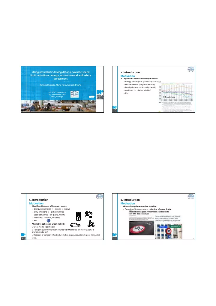
- Significant impacts of transport sector:
- Energy consumption (→ security of supply)
- GHG emissions (→ global warming)
- Local pollutants (→ air quality, health)
- Accidents (→ injuries, fatalities)
- Etc.
CO2 emissions
- 1. Introduction
Motivation
3
- Significant impacts of transport sector:
- Energy consumption (→ security of supply)
- GHG emissions (→ global warming)
- Local pollutants (→ air quality, health)
- Accidents (→ injuries, fatalities)
- Etc.
- Alternative options on urban mobility:
- Cross-modal electrification
- Transport system integration coupled with Mobility-as-a-Service (MaaS) to
promote modal shift
- Redesign of transport infrastructure (urban plazas, reduction of speed limits, etc.)
- Etc.
- 1. Introduction
Motivation
4
- Alternative options on urban mobility:
- Redesign of infrastructure → reduction of speed limits