1 a business analyst collects data about the distribution
play

1 A business analyst collects data about the distribution of hourly - PDF document

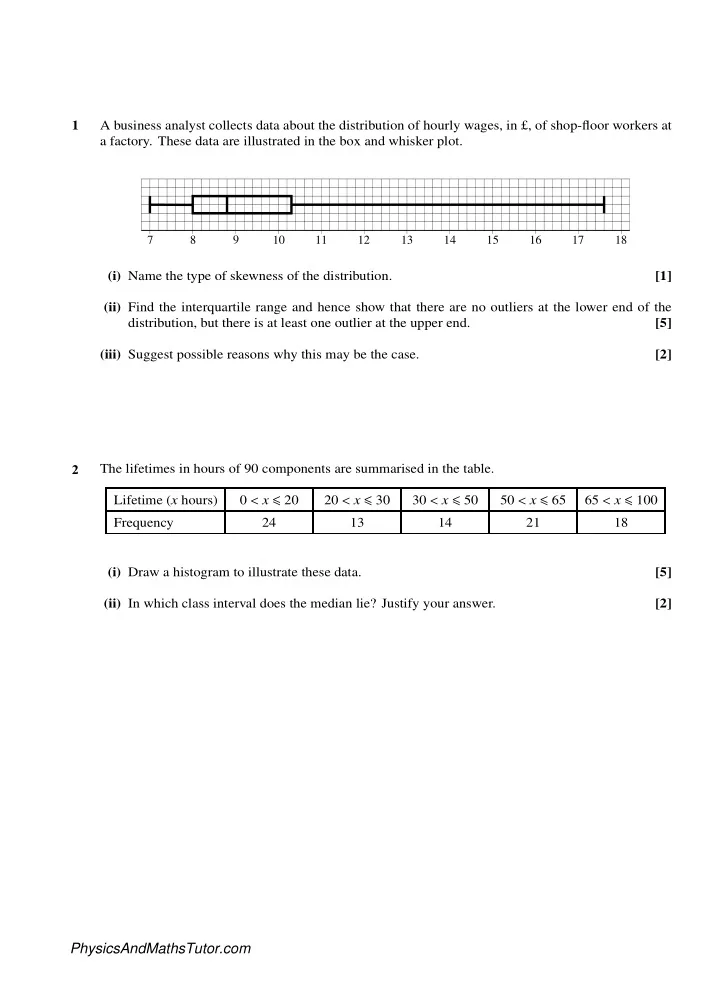
1 A business analyst collects data about the distribution of hourly wages, in , of shop-floor workers at a factory. These data are illustrated in the box and whisker plot. 7 8 9 10 11 12 13 14 15 16 17 18 (i) Name the type of


  1. 1 A business analyst collects data about the distribution of hourly wages, in £, of shop-floor workers at a factory. These data are illustrated in the box and whisker plot. 7 8 9 10 11 12 13 14 15 16 17 18 (i) Name the type of skewness of the distribution. [1] (ii) Find the interquartile range and hence show that there are no outliers at the lower end of the distribution, but there is at least one outlier at the upper end. [5] (iii) Suggest possible reasons why this may be the case. [2] 2 The lifetimes in hours of 90 components are summarised in the table. Lifetime ( x hours) 0 < x ≤ 20 20 < x ≤ 30 30 < x ≤ 50 50 < x ≤ 65 65 < x ≤ 100 Frequency 24 13 14 21 18 (i) Draw a histogram to illustrate these data. [5] (ii) In which class interval does the median lie? Justify your answer. [2] PhysicsAndMathsTutor.com

  2. 3 A pear grower collects a random sample of 120 pears from his orchard. The histogram below shows the lengths, in mm, of these pears. Frequency density 6 5 4 3 2 1 Length 0 90 0 60 70 80 100 (mm) (i) Calculate the number of pears which are between 90 and 100 mm long. [2] (ii) Calculate an estimate of the mean length of the pears. Explain why your answer is only an estimate. [4] (iii) Calculate an estimate of the standard deviation. [3] (iv) Use your answers to parts (ii) and (iii) to investigate whether there are any outliers. [4] (v) Name the type of skewness of the distribution. [1] (vi) Illustrate the data using a cumulative frequency diagram. [5] PhysicsAndMathsTutor.com

  3. 4 The frequency table below shows the distance travelled by 1200 visitors to a particular UK tourist destination in August 2008. Distance ( d miles) 0 ≤ d < 50 50 ≤ d < 100 100 ≤ d < 200 200 ≤ d < 400 Frequency 360 400 307 133 (i) Draw a histogram on graph paper to illustrate these data. [5] (ii) Calculate an estimate of the median distance. [3] PhysicsAndMathsTutor.com

Download Presentation
Download Policy: The content available on the website is offered to you 'AS IS' for your personal information and use only. It cannot be commercialized, licensed, or distributed on other websites without prior consent from the author. To download a presentation, simply click this link. If you encounter any difficulties during the download process, it's possible that the publisher has removed the file from their server.

Recommend


More recommend