y i y n median the midpoint of a group of data uchechukwu
play

y i y = n Median : the midpoint of a group of data. Uchechukwu - PDF document

ES 240: Scientific and Engineering Computation. ES 240: Scientific and Engineering Computation. Chapter 13: Linear Regression Chapter 13: Linear Regression Measure of Location Measure of Location Arithmetic mean : the sum of the individual


  1. ES 240: Scientific and Engineering Computation. ES 240: Scientific and Engineering Computation. Chapter 13: Linear Regression Chapter 13: Linear Regression Measure of Location Measure of Location � Arithmetic mean : the sum of the individual data points ( y i ) divided by the number of points n : ∑ y i y = n � Median : the midpoint of a group of data. Uchechukwu Ofoegbu Temple University � Mode : the value that occurs most frequently in a group of 13. 1: Statistical Review data. ES 240: Scientific and Engineering Computation. Chapter 13: Linear Regression ES 240: Scientific and Engineering Computation. Chapter 13: Linear Regression Measures of Spread Measures of Spread 
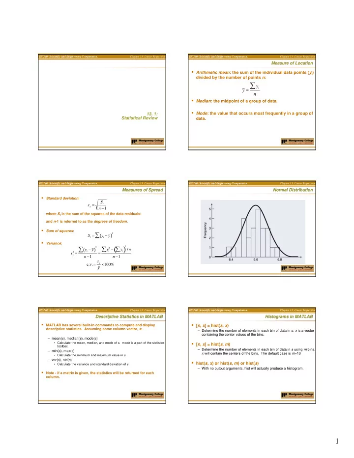
Normal Distribution Normal Distribution � Standard deviation : S t s y = n − 1 where S t is the sum of the squares of the data residuals: and n -1 is referred to as the degrees of freedom . � Sum of squares : ∑ ( ) 2 S t = y i − y � Variance : 2 − ( ) ∑ ∑ ∑ 2 ( ) 2 y i − y y i y i / n 2 = = s y n − 1 n − 1 c.v. = s y y × 100% ES 240: Scientific and Engineering Computation. Chapter 13: Linear Regression ES 240: Scientific and Engineering Computation. Chapter 13: Linear Regression Descriptive Statistics in MATLAB Descriptive Statistics in MATLAB Histograms in MATLAB Histograms in MATLAB � MATLAB has several built-in commands to compute and display � [ n , x ] = hist( s , x ) descriptive statistics. Assuming some column vector, s : – Determine the number of elements in each bin of data in s . x is a vector containing the center values of the bins. – mean( s ), median( s ), mode( s ) � [ n , x ] = hist( s , m ) • Calculate the mean, median, and mode of s . mode is a part of the statistics toolbox. – Determine the number of elements in each bin of data in s using m bins. – min( s ), max( s ) x will contain the centers of the bins. The default case is m =10 • Calculate the minimum and maximum value in s . – var( s ), std( s ) � hist( s , x ) or hist( s , m ) or hist( s ) • Calculate the variance and standard deviation of s – With no output arguments, hist will actually produce a histogram. � Note - if a matrix is given, the statistics will be returned for each column. 1

  2. ES 240: Scientific and Engineering Computation. ES 240: Scientific and Engineering Computation. Chapter 13: Linear Regression Chapter 13: Linear Regression Linear Least Linear Least- -Squares Regression Squares Regression � Linear least-squares regression is a method to determine the “best” coefficients in a linear model for given data set. � “Best” for least-squares regression means minimizing the sum of the squares of the estimate residuals. For a straight line model, this gives: n n ( ) ∑ ∑ = = − − 2 2 S e y a a x Uchechukwu Ofoegbu r i i 0 1 i = = i 1 i 1 Temple University = a int ercept 13. 2: 0 Linear Least Squares Regression = a slope 1 � This method will yield a unique line for a given set of data. ES 240: Scientific and Engineering Computation. Chapter 13: Linear Regression ES 240: Scientific and Engineering Computation. Chapter 13: Linear Regression Least- Least -Squares Fit of a Straight Line Squares Fit of a Straight Line Example Example � Using the model: ∑ ∑ ∑ − ( ) − 360 ( ) 5135 ( ) V F n x i y i x i y i = 8 312850 a 1 = = 19.47024 (m/s) (N) ( ) y = a 0 + a 1 x ∑ ∑ ( ) − 360 ( ) 2 2 − 2 8 20400 n x i x i i x i y i (x i ) 2 x i y i ( ) = − 234.2857 a 0 = y − a 1 x = 641.875 − 19.47024 45 the slope and intercept producing the best fit can be 1 10 25 100 250 est = − 234.2857 + 19.47024 v F found using: 2 20 70 400 1400 3 30 380 900 11400 ∑ ∑ ∑ 4 40 550 1600 22000 − n x i y i x i y i a 1 = 5 50 610 2500 30500 ( ) ∑ ∑ 2 − 2 n x i x i 6 60 1220 3600 73200 a 0 = y − a 1 x 7 70 830 4900 58100 8 80 1450 6400 116000 Σ 360 5135 20400 312850 ES 240: Scientific and Engineering Computation. Chapter 13: Linear Regression ES 240: Scientific and Engineering Computation. Chapter 13: Linear Regression Quantification of Error Quantification of Error Standard Error of the Estimate Standard Error of the Estimate � Regression data showing (a) the spread of data around the mean of � Recall for a straight line, the sum of the squares of the estimate the dependent data and (b) the spread of the data around the best residuals: fit line: n n ∑ ∑ ( ) S r = = y i − a 0 − a 1 x i 2 2 e i i = 1 i = 1 � Standard error of the estimate: � The reduction in spread represents the improvement due to linear regression. S r s y / x = n − 2 2

  3. ES 240: Scientific and Engineering Computation. ES 240: Scientific and Engineering Computation. Chapter 13: Linear Regression Chapter 13: Linear Regression Goodness of Fit Goodness of Fit Example Example � C oefficient of determination – the difference between the sum of the squares of the data residuals and V F est = − 234.2857 + 19.47024 v F the sum of the squares of the estimate residuals, normalized by the sum (m/s) (N) ∑ of the squares of the data residuals: ( ) S t = y i − y 2 = 1808297 (y i - ȳ ) 2 i x i y i a 0 +a 1 x i (y i -a 0 -a 1 x i ) 2 r 2 = S t − S r ∑ ( ) S r = y i − a 0 − a 1 x i = 216118 1 10 25 -39.58 380535 4171 2 S t � r 2 represents the percentage of the original uncertainty 2 20 70 155.12 327041 7245 1808297 s y = = 508.26 explained by the model. 3 30 380 349.82 68579 911 8 − 1 4 40 550 544.52 8441 30 216118 � For a perfect fit, S r =0 and r 2 =1. s y / x = = 189.79 8 − 2 5 50 610 739.23 1016 16699 r 2 = 1808297 − 216118 � If r 2 =0, there is no improvement over simply picking the mean. 6 60 1220 933.93 334229 81837 = 0.8805 1808297 7 70 830 1128.63 35391 89180 � If r 2 <0, the model is worse than simply picking the mean! 88.05% of the original uncertainty 8 80 1450 1323.33 653066 16044 has been explained by the Σ 360 5135 1808297 216118 linear model ES 240: Scientific and Engineering Computation. Chapter 13: Linear Regression ES 240: Scientific and Engineering Computation. Chapter 13: Linear Regression Nonlinear Relationships Nonlinear Relationships � Linear regression is predicated on the fact that the relationship between the dependent and independent variables is linear - this is not always the case. � Three common examples are: Uchechukwu Ofoegbu β = α x exponentia l : y e 1 Temple University 1 13. 3: Linearization of Nonlinear Relationships Linearization of Nonlinear Relationships = α β power : y x 2 2 x = α saturation - growth - rate : y β + 3 x 3 ES 240: Scientific and Engineering Computation. Chapter 13: Linear Regression ES 240: Scientific and Engineering Computation. Chapter 13: Linear Regression Linearization Linearization Transformation Examples Transformation Examples � One option for finding the coefficients for a nonlinear fit is to linearize it. For the three common models, this may involve taking logarithms or inversion: Model Nonlinear Linearized y = α 1 e β 1 x ln y = ln α 1 + β 1 x exponential : y = α 2 x β 2 log y = log α 2 + β 2 log x power : + β 3 x y = 1 1 1 y = α 3 saturation -growth - rate : β 3 + x α 3 α 3 x 3

  4. ES 240: Scientific and Engineering Computation. ES 240: Scientific and Engineering Computation. Chapter 13: Linear Regression Chapter 13: Linear Regression Example Example � Ex 13.7 Uchechukwu Ofoegbu Temple University 13. 4: Linear Regression in Matlab Linear Regression in Matlab ES 240: Scientific and Engineering Computation. Chapter 13: Linear Regression ES 240: Scientific and Engineering Computation. Chapter 13: Linear Regression Lab Lab MATLAB Functions MATLAB Functions � Ex 13.5 � Linregr function � MATLAB has a built-in function polyfit that fits a least-squares nth – Solve the problem by hand and using the linregr function order polynomial to data : and compare – p = polyfit( x , y , n ) • x : independent data • y : dependent data • n : order of polynomial to fit • p : coefficients of polynomial f ( x )= p 1 x n + p 2 x n -1 +…+ p n x + p n +1 � MATLAB’s polyval command can be used to compute a value using the coefficients. – y = polyval( p , x ) 4

Download Presentation
Download Policy: The content available on the website is offered to you 'AS IS' for your personal information and use only. It cannot be commercialized, licensed, or distributed on other websites without prior consent from the author. To download a presentation, simply click this link. If you encounter any difficulties during the download process, it's possible that the publisher has removed the file from their server.

Recommend


More recommend