Announcements Wednesday, November 28 Please fill out your CIOS - PowerPoint PPT Presentation

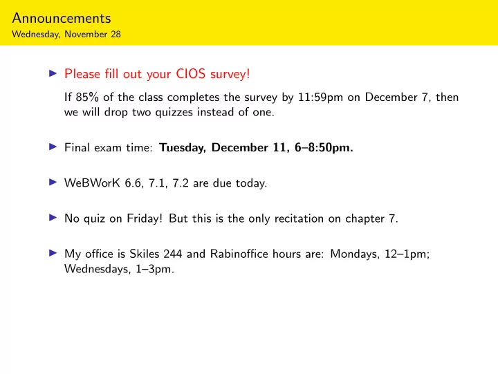
Announcements Wednesday, November 28 ◮ Please fill out your CIOS survey! If 85% of the class completes the survey by 11:59pm on December 7, then we will drop two quizzes instead of one. ◮ Final exam time: Tuesday, December 11, 6–8:50pm. ◮ WeBWorK 6.6, 7.1, 7.2 are due today. ◮ No quiz on Friday! But this is the only recitation on chapter 7. ◮ My office is Skiles 244 and Rabinoffice hours are: Mondays, 12–1pm; Wednesdays, 1–3pm.

Section 7.5 The Method of Least Squares

Motivation We now are in a position to solve the motivating problem of this third part of the course: Problem Suppose that Ax = b does not have a solution. What is the best possible approximate solution? To say Ax = b does not have a solution means that b is not in Col A . The closest possible � b for which Ax = � b does have a solution is � b = b Col A . x = � Then A � b is a consistent equation. x = � A solution � x to A � b is a least squares solution.

Least Squares Solutions Let A be an m × n matrix. Definition x in R n such that A least squares solution of Ax = b is a vector � � b − A � x � ≤ � b − Ax � for all x in R n . b Ax Note that b − A � x Ax [interactive] is in (Col A ) ⊥ . b − A � x Ax Col A x = � A � b = b Col A In other words, a least squares solution � x solves Ax = b as closely as possible . x in R n such that Equivalently, a least squares solution to Ax = b is a vector � x = � A � b = b Col A . This is because � x = � b is the closest vector to b such that A � b is consistent.

Least Squares Solutions Computation x = � We want to solve A � b = b Col A . Or, A � x = b W for W = Col A . To compute b W we need to solve A T Av = A T b ; then b W = Av . x is just a solution of A T Av = A T b ! Conclusion: � Theorem The least squares solutions of Ax = b are the solutions of ( A T A ) � x = A T b . x directly, without computing � Note we compute � b first.

Least Squares Solutions Example Find the least squares solutions of Ax = b where:     0 1 6  .    A = 1 1 b = 0 2 1 0 We have �   � 0 � 5 � 0 1 1 2 3 A T A =  =  1 1 1 1 1 3 3 2 1 and �   � 0 � 0 � 6 1 2 A T b =  =  0 . 1 1 1 6 0 Row reduce: � 5 � � 1 � 3 0 0 − 3 . 3 3 6 0 1 5 � − 3 � So the only least squares solution is � x = . 5

Least Squares Solutions Example, continued How close did we get?     � − 3 � 0 1 5 �     b = A � x = 1 1 = 2 5 2 1 − 1 The distance from b is � � � �       � � � � 6 5 1 � √ � � � � 1 2 + ( − 2) 2 + 1 2 = �  − � � �      � b − A � x � = 0 2 = − 2 = 6 . � � � � � � � � 0 − 1 1 [interactive] Note that b � � 5 v 2 − 3 v 1 − 3 v 1 √ 6 5 v 2 records the coefficients � � of v 1 and v 2 in � − 3 b . b Col( A ) = A Col A 5

Least Squares Solutions Second example Find the least squares solutions of Ax = b where:     2 0 1  .    A = − 1 1 b = 0 0 2 − 1 We have �   � 2 � � 2 0 − 1 0 5 − 1 A T A =  =  − 1 1 0 1 2 − 1 5 0 2 and �   � 2 � 2 � 1 − 1 0 A T b =  =  0 . 0 1 2 − 2 − 1 Row reduce: � � � 1 � 5 − 1 2 0 1 / 3 . − 1 5 − 2 0 1 − 1 / 3 � 1 / 3 � So the only least squares solution is � x = . [interactive] − 1 / 3

Least Squares Solutions Uniqueness When does Ax = b have a unique least squares solution � x ? Theorem Let A be an m × n matrix. The following are equivalent: 1. Ax = b has a unique least squares solution for all b in R n . 2. The columns of A are linearly independent. 3. A T A is invertible. In this case, the least squares solution is ( A T A ) − 1 ( A T b ). x = � Why? If the columns of A are linearly de pendent, then A � b has many solutions: b v 2 v 1 [interactive] v 3 � b = A � x Col A Note: A T A is always a square matrix, but it need not be invertible.

Application Data modeling: best fit line Find the best fit line through (0 , 6), (1 , 0), and (2 , 0). [interactive] The general equation of a line is (0 , 6) y = C + Dx . 1 So we want to solve: 6 = C + D · 0 y = 0 = C + D · 1 − 3 0 = C + D · 2 . x + 5 In matrix form: − 2     � C � (2 , 0) 1 0 6     . 1 1 = 0 (1 , 0) 1 D 1 2 0 We already saw: the least squares solution is     � 5 � � � 6 1 . So the best fit line is 5 − 3   =   0 − 2 A − − 3 0 1 y = − 3 x + 5 .

Poll Poll What does the best fit line minimize? A. The sum of the squares of the distances from the data points to the line. B. The sum of the squares of the vertical distances from the data points to the line. C. The sum of the squares of the horizontal distances from the data points to the line. D. The maximal distance from the data points to the line. Answer: B. See the picture on the previous slide.

Application Best fit ellipse Find the best fit ellipse for the points (0 , 2), (2 , 1), (1 , − 1), ( − 1 , − 2), ( − 3 , 1), ( − 1 , − 1). The general equation for an ellipse is x 2 + Ay 2 + Bxy + Cx + Dy + E = 0 So we want to solve: (0) 2 + A (2) 2 + B (0)(2) + C (0) + D (2) + E = 0 (2) 2 + A (1) 2 + B (2)(1) + C (2) + D (1) + E = 0 (1) 2 + A ( − 1) 2 + B (1)( − 1) + C (1) + D ( − 1) + E = 0 ( − 1) 2 + A ( − 2) 2 + B ( − 1)( − 2) + C ( − 1) + D ( − 2) + E = 0 ( − 3) 2 + A (1) 2 + B ( − 3)(1) + C ( − 3) + D (1) + E = 0 ( − 1) 2 + A ( − 1) 2 + B ( − 1)( − 1) + C ( − 1) + D ( − 1) + E = 0 In matrix form:     4 0 0 2 1   0 A     1 2 2 1 1 − 4       B       1 − 1 1 − 1 1 − 1       C = .       4 2 − 1 − 2 1 − 1       D     1 − 3 − 3 1 1 − 9 E 1 1 − 1 − 1 1 − 1

Application Best fit ellipse, continued     4 0 0 2 1 0 1 2 2 1 1 − 4         1 − 1 1 − 1 1 − 1     A = b = .     4 2 − 1 − 2 1 − 1         1 − 3 − 3 1 1 − 9 1 1 − 1 − 1 1 − 1     36 7 − 5 0 12 − 19  7 19 9 − 5 1   17      A T A = A T b = − 5 9 16 1 − 2 20         0 − 5 1 12 0 − 9 12 1 − 2 0 6 − 16 Row reduce:     36 7 − 5 0 12 − 19 1 0 0 0 0 405 / 266 7 19 9 − 5 1 17 0 1 0 0 0 − 89 / 133         − 5 9 16 1 − 2 20 0 0 1 0 0 201 / 133         0 − 5 1 12 0 − 9 0 0 0 1 0 − 123 / 266 12 1 − 2 0 6 − 16 0 0 0 0 1 − 687 / 133 Best fit ellipse: x 2 + 405 266 y 2 − 89 133 xy + 201 133 x − 123 266 y − 687 133 = 0 or 266 x 2 + 405 y 2 − 178 xy + 402 x − 123 y − 1374 = 0 .

Application Best fit ellipse, picture [interactive] (0 , 2) ( − 3 , 1) (2 , 1) ( − 1 , 1) (1 , − 1) ( − 1 , − 2) 266 x 2 + 405 y 2 − 178 xy + 402 x − 123 y − 1374 = 0 Remark: Gauss invented the method of least squares to do exactly this: he predicted the (elliptical) orbit of the asteroid Ceres as it passed behind the sun in 1801.

Application Best fit parabola What least squares problem Ax = b finds the best parabola through the points ( − 1 , 0 . 5), (1 , − 1), (2 , − 0 . 5), (3 , 2)? The general equation for a parabola is y = Ax 2 + Bx + C . So we want to solve: 0 . 5 = A ( − 1) 2 + B ( − 1) + C A (1) 2 + − 1 = B (1) + C A (2) 2 + − 0 . 5 = B (2) + C A (3) 2 + 2 = B (3) + C In matrix form:       1 − 1 1 0 . 5 A     1 1 1 − 1  =       . B    4 2 1 − 0 . 5 C 9 3 1 2 88 y = 53 x 2 − 379 Answer: 5 x − 82

Application Best fit parabola, picture 88 y = 53 x 2 − 379 5 x − 82 (3 , 2) ( − 1 , 0 . 5) (2 , − 0 . 5) (1 , − 1) [interactive]

Application Best fit linear function x y f ( x , y ) What least squares problem Ax = b finds the best 1 0 0 linear function f ( x , y ) fitting the following data? 0 1 1 The general equation for a linear function in two − 1 0 3 variables is 0 − 1 4 f ( x , y ) = Ax + By + C . So we want to solve A (1) + B (0) + C = 0 A (0) + B (1) + C = 1 A ( − 1) + B (0) + C = 3 A (0) + B ( − 1) + C = 4 In matrix form:       1 0 1 0 A     0 1 1 1     =    . B    − 1 0 1 3 C 0 − 1 1 4 f ( x , y ) = − 3 2 x − 3 Answer: 2 y + 2

Application Best fit linear function, picture [interactive] f ( − 1 , 0) (0 , − 1 , 4) f ( x , y ) ( − 1 , 0 , 3) f (0 , − 1) Graph of f ( x , y ) = − 3 2 x − 3 2 y + 2 (0 , 1 , 1) y f (1 , 0) x f (0 , 1) (1 , 0 , 0)