[ ] Wu et al. (2000): ( ) b = + 1 1 b 2 Requires - PowerPoint PPT Presentation

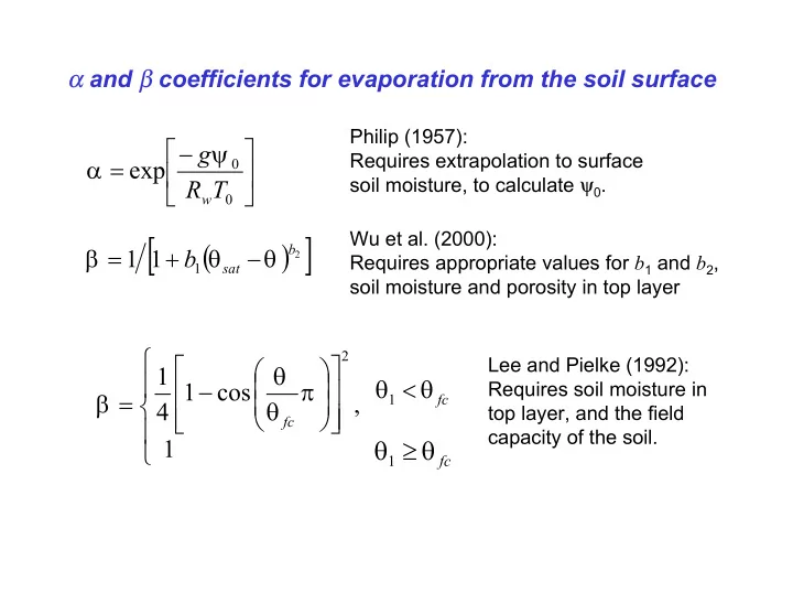
α and β coefficients for evaporation from the soil surface Philip (1957): −  ψ g Requires extrapolation to surface α = exp 0   soil moisture, to calculate ψ 0 . R T   w 0 [ ] Wu et al. (2000): ( ) b β = + θ − θ 1 1 b 2 Requires appropriate values for b 1 and b 2 , 1 sat soil moisture and porosity in top layer  2   Lee and Pielke (1992):   θ 1    θ < θ − π   1 cos Requires soil moisture in β =   ,  1 fc θ 4   top layer, and the field     fc  capacity of the soil. θ ≥ θ 1  1 fc

Canopy Conductance in CLASS 2.x • g c scales linearly with leaf area index ( Λ ) [ ] ( ) Λ = Λ Λ g g c c , max max • employs the multiplicative Jarvis-Stewart approach to represent the response to environmental stresses ) ( ( ) ( ) ( ) = ∆ ψ ˆ g g f K f e f f T 1 2 3 4 c c ↓ s , r a where: ( ) Λ ˆ g g is a composite value of over the 4 vegetation groups c c K ↓ is incoming solar radiation ∆ e is vapour pressure deficit ψ s,r is soil water suction in the rooting zone T a is air temperature

Canopy Conductance in CLASS 2.x • g c,max is hard coded as 20 mm·s -1 for all vegetation types • functions f 1 - f 4 are the same for all vegetation types ( ) ( ) ( ) ( ) = ∆ ψ ˆ g g f K f e f f T c c 1 ↓ 2 3 s , r 4 a 1.2 1.0 0.8 1.2 f ( T a ) 0.6 1.0 0.4 0.8 1.2 0.2 f ( K ↓ ) 0.6 1.0 1.2 0.0 0.4 0.8 -10 0 10 20 30 40 50 1.0 f ( ∆ e ) 0.2 0.6 T a (°C) 0.8 0.0 0.4 f ( ψ ) 0.6 0 250 500 750 1000 0.2 0.4 K ↓ (W·m -2 ) 0.0 0.2 0 1 2 3 4 0.0 ∆ e (kPa) 0.0 -0.5 -1.0 -1.5 -2. ψ (MPa)

Canopy Conductance in CLASS 3.0 Following papers by Schulze, Kelliher, Leuning and Raupach (1995): •The maximum unstressed stomatal conductance is g s,max • We model a hyperbolic response to solar radiation 1.2 g Q 1.0 = s , max ↓ g 0.8 s + Q Q f ( Q ↓ ) 0.6 ↓ l 1 / 2 0.4 where: 0.2 0.0 Q ↓ is incoming photosynthetically active radiation, 0 250 500 750 1000 Q l 1/2 is the value of Q ↓ where g s = g s,max /2 Q ↓ (W·m -2 )

Canopy Conductance in CLASS 3.0 • Assuming photosynthetically active radiation at height h ( Q h ) declines exponentially through the canopy with cumulative leaf area index ( ξ ) ( ) = − ξ Q Q ↓ exp c h Q where c Q is an extinction coefficient • Differentiating with respect to ξ and assuming that g c is the parallel sum of g s through the canopy, we can combine the previous two equations to yield   + g Q Q = s , max ↓ 1 / 2 g ln   ( ) c − Λ + c Q exp c Q     Q Q 1 / 2 ↓ which is canopy conductance in the absence of stress caused by humidity, water availability and air temperature

Canopy Conductance in CLASS 3.0 • We can represent stress caused by humidity, water availability and temperature using multiplicative functions, as   + g Q Q ( ) ( ) ( ) = ⋅ ∆ ⋅ ψ ⋅ s , max 1 / 2 ↓ g ln f e f f T   ( ) c s , r a − Λ + c Q exp c Q     Q Q 1 / 2 ↓ • To represent various vegetation types, f ( ∆ e ) and f ( ψ s,r ) have adjustable coefficients that, along with Q 1/2 , can be read from the initialization file, while default values are provided for major vegetation categories.

Canopy Conductance in CLASS 3.0 • To prevent step changes in CLASS’s output: • f ( T a ) has been changed, • The step change at a wilting point has been removed using more gradual bounds. from f ( ψ s,r ) 1.2 1.2 CLASS 2 1.0 1.0 CLASS 3 0.8 0.8 Previous f ( T a ) f ( ψ ) wilting point 0.6 0.6 0.4 0.4 0.2 CLASS 2 0.2 CLASS 3 0.0 0.0 -10 0 10 20 30 40 50 0.0 -0.5 -1.0 -1.5 -2.0 ψ (MPa) T a (°C)

Partitioning Rainfall and Snowfall In CLASS 3.0 1 . 0 S t e p c h a n g e G r a d u a l l i n e a r 0 . 8 P o l y n o m i a l s n o w 0 . 6 0 . 4 f 0 . 2 0 . 0 - 6 - 4 - 2 0 2 4 6 8 1 0 A i r t e m p e r a t u r e ( ° C ) • CLASS 2 employed a step change function: Air temperature ≤ 0 °C → Snow Air temperature > 0 °C → Rain • CLASS 3 provides a choice of three functions: 1. The step change function from CLASS 2 2. A gradual linear change between 0 and 2 ° C 3. A polynomial based on Auer (1974) and recommended by Fassnacht.

Fresh Snow Density In CLASS 3 2 2 5 ( k g · m C L A S S 2 ) 2 0 0 - 3 C L A S S 3 1 7 5 f r e s h s n o w 1 5 0 1 2 5 1 0 0 7 5 ρ 5 0 - 1 0 - 8 - 6 - 4 - 2 0 2 4 6 8 A i r t e m p e r a t u r e ( ° C ) • CLASS 2 assumed a constant snow density of 100 kg·m -3 . • CLASS 3 employs a variable density based on air temperature.

Maximum Snow Density In CLASS 3 ( k g · m ) - 3 7 0 0 6 0 0 m a x i m u m s n o w 5 0 0 4 0 0 ρ 3 0 0 T s n o w < 0 ° C 2 0 0 T s n o w = 0 ° C 1 0 0 0 . 0 0 . 5 1 . 0 1 . 5 2 . 0 S n o w d e p t h ( m ) • In CLASS 2, the maximum density that a snow- pack could achieve in the absence of melting, was set to 300 kg·m -3 . • In CLASS 3, the maximum density that a snow- pack can achieve in the absence of melting varies with snow depth, and is larger for a snowpack at a temperature of 0 °C than for a colder snowpack.

Snow Interception In CLASS 3 • If we define snow interception ( I ) as snow that falls the canopy, I is found as: the rate of snowfall x (1 – the sky view factor), • In CLASS 2, all intercepted snow stayed on the canopy until until the interception capacity ( I *) was reached. I * for water and snow was 0.2· LAI (in kg·m -2 ). However, snow acts as a bridge between branches and between conifer needles. Hedstrom and Pomeroy (1998) have shown that the average I * is about 0.5· LAI . • In CLASS 3, I * = 6· LAI ·(0.27+46/ ρ fresh snow )

Snow Interception In CLASS 3 • In CLASS 3, not all of the intercepted snow stays on the canopy. • Snow added to the canopy interception store ( S load ) is found as:   I ∆ ( )  T  −   = ⋅ * − − * S 0 . 697   I I 1 e I load   0  3600    where 0.697 is a dimensionless snow unloading coefficient, ∆ T is the model time step in seconds, and I 0 is the initial amount of snow stored on the canopy. • Not all of the intercepted snow (I.e. snow that lands on the canopy) stays on the canopy. This snow that falls or drips from the canopy is found as: I – S load.

Schematic representation of aerodynamic resistances to the transfer of momentum and to the transfer of scalar properties, showing the excess resistance r b due to molecular effects and the relation between the surface temperature θ 0 and the temperature θ ( z 0 ). (From J.R. Garratt, “The Atmospheric Boundary Layer”)

Q H,T ( T a,c – T a ) = Q H,c ( T c – T a,c ) + Q H,g ( T g – T a,c ) Q H,T Q H,c Q H,g Schematic representation of the main elements of a non-isothermal or two- component canopy model. Linked to the atmosphere (via resistances r s , r b and r a ), to the soil or undergrowth (via resistance r d ) and the deep soil (via evapotranspiration), the canopy and upper soil layer are at temperatures T f and T g . P g is the precipitation reaching the soil surface. (From J.R. Garratt, “The Atmospheric Boundary Layer”)

Grid-cell averages calculated ( ) ∑ ( ) = X i X i , m m X( i, 1) X( i, 2) X( i, 3) Prognostic variable arrays scattered back onto original matrix grid X ′ (( i -1)· nm +1) X ′ (( i -1)· nm +2) X ′ (( i -1)· nm +3) CLASS Patch 1 Patch 2 Patch 3 Prognostic variable matrix arrays gathered from mosaic grid onto vector array For the i th grid-cell: X( i, 1) X( i, 2) X( i, 3) • ni is the number of grid elements (grid cells) • nm is the number of mosaic elements (patches in each grid-cell)