
SLIDE 1
- 1-
Workshop 8.2a: Heterogeneity
Murray Logan
July 23, 2016
Table of contents
1 Linear modelling assumptions 1 2 Heteroscadacity in ANOVA 12 3 Worked Examples 17
- 1. Linear modelling assumptions
1.1. Assumptions
yi = β0 + β1 × xi + εi ϵi ∼ N(0, σ2)
1.2. Linear modelling assumptions
yi = β0 + β1 × xi + εi ϵi ∼ N(0, σ2)
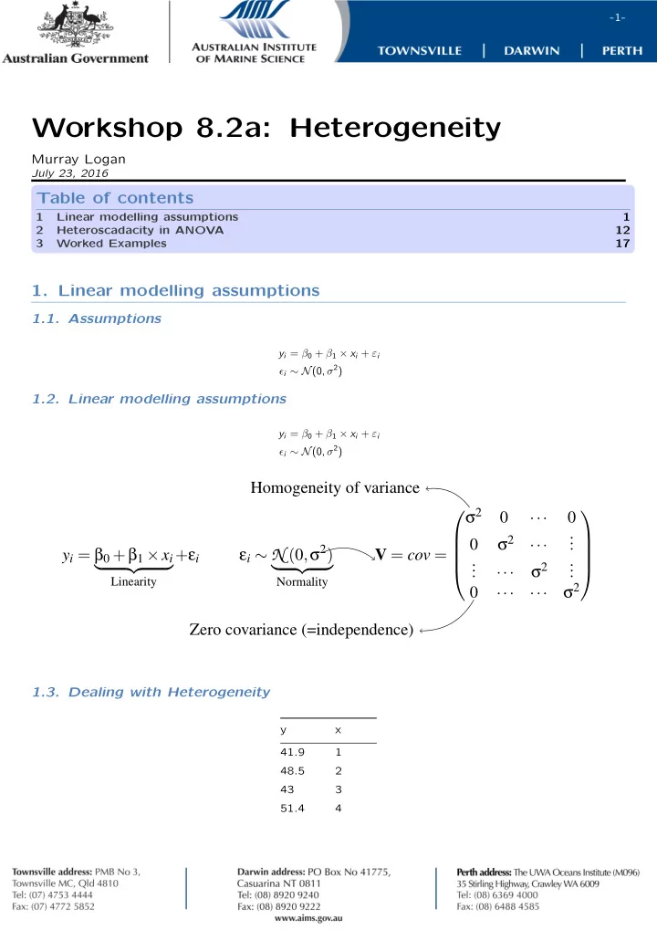
yi = β0 +β1 ×xi
- Linearity
+εi εi ∼ N (0,. σ2)
- Normality
. V = cov = . σ2 ··· σ2 ··· . . . . . . ··· σ2 . . . . ··· ··· σ2 . Homogeneity of variance . Zero covariance (=independence) .
1.3. Dealing with Heterogeneity
y x 41.9 1 48.5 2 43 3 51.4 4