
SLIDE 1
- 1-
Workshop 10.4: Generalized linear models
Murray Logan
August 16, 2016
Table of contents
1 Exponential family distributions 2
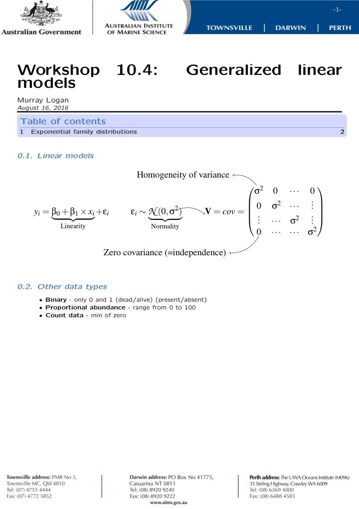
0.1. Linear models
yi = β0 +β1 ×xi
- Linearity
+εi εi ∼ N (0,. σ2)
- Normality
. V = cov = . σ2 ··· σ2 ··· . . . . . . ··· σ2 . . . . ··· ··· σ2 . Homogeneity of variance . Zero covariance (=independence) .
0.2. Other data types
- Binary - only 0 and 1 (dead/alive) (present/absent)
- Proportional abundance - range from 0 to 100
- Count data - min of zero