Workshop 7: (Generalized) Linear models Murray Logan July 19, - - PDF document

• 1-

Workshop 7: (Generalized) Linear models

Murray Logan

July 19, 2017

Table of contents

1 Linear model Assumptions 1 2 Multiple (Genearalized) Linear Regression 15 3 Centering data 17 4 Assumptions 20 5 Multiple linear models in R 21 6 Model selection 26 7 Worked Examples 27 8 Anova Parameterization 29 9 Partitioning of variance (ANOVA) 35 10 Worked Examples 37

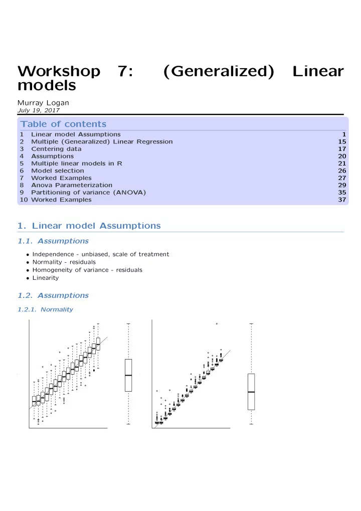
• 1. Linear model Assumptions

1.1. Assumptions

• Independence - unbiased, scale of treatment
• Normality - residuals
• Homogeneity of variance - residuals
• Linearity

1.2. Assumptions

1.2.1. Normality

• y
• y

• 5

10 15 20 25 30 0.0 0.5 1.0 1.5 2.0 2.5

• 5

10 15 20 25 30 0.0 0.5 1.0 1.5 2.0 2.5

• 2-

1.3. Assumptions

1.3.1. Homogeneity of variance

• ●
• ●
• ●
• y

X Y

• ● ●
• ●
• x

y

• ●
• res

Predicted x Residuals

• ●
• ●
• ●
• y

X Y

• x

y

• res

Predicted x Residuals 1.4. Assumptions

1.4.1. Linearity Trendline

• 5

10 15 20 25 30 10 20 30 40 50 60

• 5

10 15 20 25 30 0.0 0.5 1.0 1.5 2.0 2.5

1.5. Assumptions

1.5.1. Linearity Loess (lowess) smoother

• 3-
• 5

10 15 20 25 30 10 20 30 40 50 60

• 5

10 15 20 25 30 0.0 0.5 1.0 1.5 2.0 2.5

1.6. Assumptions

1.6.1. Linearity Spline smoother

• 4-
• 5

10 15 20 25 30 10 20 30 40 50 60

• 5

10 15 20 25 30 0.0 0.5 1.0 1.5 2.0 2.5

1.7. Assumptions

yi = β0 + β1 × xi + εi ϵi ∼ N(0, σ2)

1.8. Assumptions

yi = β0 + β1 × xi + εi ϵi ∼ N(0, σ2)

1.9. The linear predictor

y = β0 + β1x Y X 3 2.5 1 6 2 5.5 3 9 4 8.6 5 12 6 3.0 = β0 × 1 + β1 × 0 2.5 = β0 × 1 + β1 × 1 6.0 = β0 × 1 + β1 × 2 5.5 = β0 × 1 + β1 × 3 9.0 = β0 × 1 + β1 × 4 8.6 = β0 × 1 + β1 × 5 12.0 = β0 × 1 + β1 × 6

• 5-

          3.0 2.5 6.0 5.5 9.0 8.6 12.0          

• Response values

=           1 1 1 1 2 1 3 1 4 1 5 1 6          

• Model matrix

× (β0 β1 )

Parameter vector

1.10. Linear models in R

> lm(formula, data= DATAFRAME)

Model R formula Description yi = β0 + β1xi y~1+x y~x Full model yi = β0 y~1 Null model yi = β1 y~-1+x Through origin

> lm(Y~X, data= DATA)

Call: lm(formula = Y ~ X, data = DATA) Coefficients: (Intercept) X 2.136 1.507

1.11. Linear models in R

> Xmat = model.matrix(~X, data=DATA) > Xmat

(Intercept) X 1 1 0 2 1 1 3 1 2 4 1 3 5 1 4 6 1 5 7 1 6 attr(,"assign") [1] 0 1

> lm.fit(Xmat,DATA$Y)

$coefficients (Intercept) X 2.135714 1.507143

• 6-

$residuals [1] 0.8642857 -1.1428571 0.8500000 -1.1571429 0.8357143 -1.0714286 0.8214286 $effects (Intercept) X

• 17.6131444

7.9750504 0.6507186

• 1.5697499

0.2097817

• 1.9106868
• 0.2311552

$rank [1] 2 $fitted.values [1] 2.135714 3.642857 5.150000 6.657143 8.164286 9.671429 11.178571 $assign [1] 0 1 $qr $qr (Intercept) X 1

• 2.6457513 -7.93725393

2 0.3779645 5.29150262 3 0.3779645 0.03347335 4 0.3779645 -0.15550888 5 0.3779645 -0.34449112 6 0.3779645 -0.53347335 7 0.3779645 -0.72245559 attr(,"assign") [1] 0 1 $qraux [1] 1.377964 1.222456 $pivot [1] 1 2 $tol [1] 1e-07 $rank [1] 2 attr(,"class") [1] "qr" $df.residual [1] 5

1.12. Example

1.12.1. Linear Model yi = β0 + β1xi N(0, σ2)

> DATA.lm<-lm(Y~X, data=DATA)

• 7-

1.12.2. Generalized Linear Model g(yi) = β0 + β1xi N(0, σ2)

> DATA.glm<-glm(Y~X, data=DATA, family='gaussian')

1.13. Model diagnostics

1.13.1. Residuals

• 1

2 3 4 5 6

x

5 10 15 20 25 30

y

1.14. Model diagnostics

• 8-

1.14.1. Residuals

• 1

2 3 4 5 6

x

5 10 15 20 25 30

y

1.15. Model diagnostics

1.15.1. Leverage

• 5

10 15 20

x

5 10 15 20 25 30

y

• 9-

1.16. Model diagnostics

1.16.1. Cook’s D

• 5

10 15 20

x

10 20 30 40 50

y

1.17. Example

1.17.1. Model evaluation Extractor Description residuals() Extracts residuals from model

• 1

2 3 4 5 6

x

5 10 15

y

> residuals(DATA.lm)

1 2 3 4 5 6 7 0.8642857 -1.1428571 0.8500000 -1.1571429 0.8357143 -1.0714286 0.8214286

1.18. Example

• 10-

1.18.1. Model evaluation Extractor Description residuals() Extracts residuals from model fitted() Extracts the predicted values

• 1

2 3 4 5 6

x

5 10 15

y

> fitted(DATA.lm)

1 2 3 4 5 6 7 2.135714 3.642857 5.150000 6.657143 8.164286 9.671429 11.178571

1.19. Example

1.19.1. Model evaluation Extractor Description residuals() Extracts residuals from model fitted() Extracts the predicted values plot() Series of diagnostic plots

> plot(DATA.lm)

• 11-

2 4 6 8 10 −1.0 0.0 1.0 Fitted values Residuals

• Residuals vs Fitted

4 2 6

• −1.0

0.0 0.5 1.0 −1.0 0.0 1.0 Theoretical Quantiles Standardized residuals

Normal Q−Q

2 6 4

2 4 6 8 10 0.0 0.4 0.8 Fitted values Standardized residuals

• Scale−Location

2 6 4

0.0 0.1 0.2 0.3 0.4 −1.0 0.0 1.0 Leverage Standardized residuals

• Cook's distance

0.5 0.5

Residuals vs Leverage

1 7 2

1.20. Example

1.20.1. Model evaluation Extractor Description residuals() Residuals fitted() Predicted values plot() Diagnostic plots influence.measures() Leverage (hat) and Cook’s D

1.21. Example

1.21.1. Model evaluation

> influence.measures(DATA.lm)

Influence measures of lm(formula = Y ~ X, data = DATA) : dfb.1_ dfb.X dffit cov.r cook.d hat inf 1 0.9603 -7.99e-01 0.960 1.82 0.4553 0.464 2 -0.7650 5.52e-01 -0.780 1.15 0.2756 0.286 3 0.3165 -1.63e-01 0.365 1.43 0.0720 0.179 4 -0.2513 -7.39e-17 -0.453 1.07 0.0981 0.143 5 0.0443 1.60e-01 0.357 1.45 0.0696 0.179 6 0.1402 -5.06e-01 -0.715 1.26 0.2422 0.286 7 -0.3466 7.50e-01 0.901 1.91 0.4113 0.464

1.22. Example

1.22.1. Model evaluation

• 12-

Extractor Description residuals() Residuals fitted() Predicted values plot() Diagnostic plots influence.measures() Leverage, Cook’s D summary() Summarizes important output from model

1.23. Example

1.23.1. Model evaluation

> summary(DATA.lm)

Call: lm(formula = Y ~ X, data = DATA) Residuals: 1 2 3 4 5 6 7 0.8643 -1.1429 0.8500 -1.1571 0.8357 -1.0714 0.8214 Coefficients: Estimate Std. Error t value Pr(>|t|) (Intercept) 2.1357 0.7850 2.721 0.041737 * X 1.5071 0.2177 6.923 0.000965 ***

• Signif. codes:

0 '***' 0.001 '**' 0.01 '*' 0.05 '.' 0.1 ' ' 1 Residual standard error: 1.152 on 5 degrees of freedom Multiple R-squared: 0.9055, Adjusted R-squared: 0.8866 F-statistic: 47.92 on 1 and 5 DF, p-value: 0.0009648

1.24. Example

1.24.1. Model evaluation Extractor Description residuals() Residuals fitted() Predicted values plot() Diagnostic plots influence.measures() Leverage, Cook’s D summary() Model output confint() Confidence intervals of parameters

1.25. Example

• 13-

1.25.1. Model evaluation

> confint(DATA.lm)

2.5 % 97.5 % (Intercept) 0.1178919 4.153537 X 0.9474996 2.066786

1.26. Worked Examples

> fert <- read.csv('../data/fertilizer.csv', strip.white=T) > fert

FERTILIZER YIELD 1 25 84 2 50 80 3 75 90 4 100 154 5 125 148 6 150 169 7 175 206 8 200 244 9 225 212 10 250 248

> head(fert)

FERTILIZER YIELD 1 25 84 2 50 80 3 75 90 4 100 154 5 125 148 6 150 169

> summary(fert)

FERTILIZER YIELD Min. : 25.00 Min. : 80.0 1st Qu.: 81.25 1st Qu.:104.5 Median :137.50 Median :161.5 Mean :137.50 Mean :163.5 3rd Qu.:193.75 3rd Qu.:210.5 Max. :250.00 Max. :248.0

> str(fert)

'data.frame': 10 obs. of 2 variables: $ FERTILIZER: int 25 50 75 100 125 150 175 200 225 250 $ YIELD : int 84 80 90 154 148 169 206 244 212 248

• 14-

1.27. Worked Examples

Question: is there a relationship between fertilizer concentration and grass yeild? Linear model: Yi = β0 + β1Fi + εi ε ∼ N(0, σ2)

• 1. Tidy data
• 2. EDA
• 3. Fit model
• 4. Evaluate model
• 5. Summarize model

1.28. Worked Examples

> polis <- read.csv('../data/polis.csv', strip.white=T) > head(polis)

ISLAND RATIO PA 1 Bota 15.41 1 2 Cabeza 5.63 1 3 Cerraja 25.92 1 4 Coronadito 15.17 5 Flecha 13.04 1 6 Gemelose 18.85

> summary(polis)

ISLAND RATIO PA Angeldlg: 1 Min. : 0.21 Min. :0.0000 Bahiaan : 1 1st Qu.: 5.86 1st Qu.:0.0000 Bahiaas : 1 Median :15.17 Median :1.0000 Blanca : 1 Mean :18.74 Mean :0.5263 Bota : 1 3rd Qu.:23.20 3rd Qu.:1.0000 Cabeza : 1 Max. :63.16 Max. :1.0000 (Other) :13

1.29. Worked Examples

> peake <- read.csv('../data/peakquinn.csv', strip.white=T) > head(peake)

AREA INDIV 1 516.00 18 2 469.06 60 3 462.25 57 4 938.60 100 5 1357.15 48 6 1773.66 118

> summary(peake)

• 15-

AREA INDIV Min. : 462.2 Min. : 18.0 1st Qu.: 1773.7 1st Qu.: 148.0 Median : 4451.7 Median : 338.0 Mean : 7802.0 Mean : 446.9 3rd Qu.: 9287.7 3rd Qu.: 632.0 Max. :27144.0 Max. :1402.0

1.30. Worked Examples

Question: is there a relationship between mussel clump area and number of individuals? Linear model: Indivi = β0 + β1Areai + εi ε ∼ N(0, σ2) ln(Indivi) = β0 + β1ln(Areai) + εi ε ∼ N(0, σ2)

1.31. Worked Examples

Question: is there a relationship between mussel clump area and number of individuals? Linear model: Indivi ∼ Pois(λi) log(λ) = β0 + β1ln(Areai)

• 2. Multiple (Genearalized) Linear Regression

2.1. Multiple Linear Regression

2.1.1. Additive model growth = intercept + temperature + nitrogen yi = β0 + β1xi1 + β2xi2 + ... + βjxij + ϵi OR yi = β0 +

N

∑

j=1:n

βjxji + ϵi

2.2. Multiple Linear Regression

2.2.1. Additive model growth = intercept + temperature + nitrogen yi = β0 + β1xi1 + β2xi2 + ... + βjxij + ϵi

• effect of one predictor holding the other(s) constant

• 16-

2.3. Multiple Linear Regression

2.3.1. Additive model growth = intercept + temperature + nitrogen yi = β0 + β1xi1 + β2xi2 + ... + βjxij + ϵi Y X1 X2 3 22.7 0.9 2.5 23.7 0.5 6 25.7 0.6 5.5 29.1 0.7 9 22 0.8 8.6 29 1.3 12 29.4 1

2.4. Multiple Linear Regression

2.4.1. Additive model 3 = β0 + (β1 × 22.7) + (β2 × 0.9) + ε1 2.5 = β0 + (β1 × 23.7) + (β2 × 0.5) + ε2 6 = β0 + (β1 × 25.7) + (β2 × 0.6) + ε3 5.5 = β0 + (β1 × 29.1) + (β2 × 0.7) + ε4 9 = β0 + (β1 × 22) + (β2 × 0.8) + ε5 8.6 = β0 + (β1 × 29) + (β2 × 1.3) + ε6 12 = β0 + (β1 × 29.4) + (β2 × 1) + ε7

2.5. Multiple Linear Regression

2.5.1. Multiplicative model growth = intercept + temp + nitro + temp × nitro yi = β0 + β1xi1 + β2xi2 + β3xi1xi2 + ... + ϵi

2.6. Multiple Linear Regression

• 17-

2.6.1. Multiplicative model

3 = β0 + (β1 × 22.7) + (β2 × 0.9) + (β3 × 22.7 × 0.9) + ε1 2.5 = β0 + (β1 × 23.7) + (β2 × 0.5) + (β3 × 23.7 × 0.5) + ε2 6 = β0 + (β1 × 25.7) + (β2 × 0.6) + (β3 × 25.7 × 0.6) + ε3 5.5 = β0 + (β1 × 29.1) + (β2 × 0.7) + (β3 × 29.1 × 0.7) + ε4 9 = β0 + (β1 × 22) + (β2 × 0.8) + (β3 × 22 × 0.8) + ε5 8.6 = β0 + (β1 × 29) + (β2 × 1.3) + (β3 × 29 × 1.3) + ε6 12 = β0 + (β1 × 29.4) + (β2 × 1) + (β3 × 29.4 × 1) + ε7

• 3. Centering data

3.1. Multiple Linear Regression

3.1.1. Centering

• ●
• ●
• 10

20 30 40 50 60

x

−20 −10 10 20

y

3.2. Multiple Linear Regression

• 18-

3.2.1. Centering

• 47

48 49 50 51 52 53 54

3.3. Multiple Linear Regression

3.3.1. Centering

• 47

48 49 50 51 52 53 54

• 19-

3.4. Multiple Linear Regression

3.4.1. Centering

• 47

48 49 50 51 52 53 54 −3 −2 −1 1 2 3 4

3.5. Multiple Linear Regression

3.5.1. Centering

• −4

−2 2 4

cx1

16 18 20 22 24

y

• 20-
• 4. Assumptions

4.1. Multiple Linear Regression

4.1.1. Assumptions Normality, homog., linearity

4.2. Multiple Linear Regression

4.2.1. Assumptions (multi)collinearity

4.3. Multiple Linear Regression

4.3.1. Variance inflation Strength of a relationship R2 Strong when R2 ≥ 0.8

4.4. Multiple Linear Regression

4.4.1. Variance inflation var.inf = 1 1 − R2 Collinear when var.inf >= 5 Some prefer > 3

4.5. Multiple Linear Regression

4.5.1. Assumptions (multi)collinearity

> library(car) > # additive model - scaled predictors > vif(lm(y ~ cx1 + cx2, data))

cx1 cx2 1.743817 1.743817

4.6. Multiple Linear Regression

4.6.1. Assumptions (multi)collinearity

> library(car) > # additive model - scaled predictors > vif(lm(y ~ cx1 + cx2, data))

• 21-

cx1 cx2 1.743817 1.743817

> # multiplicative model - raw predictors > vif(lm(y ~ x1 * x2, data))

x1 x2 x1:x2 7.259729 5.913254 16.949468

4.7. Multiple Linear Regression

4.7.1. Assumptions

> # multiplicative model - raw predictors > vif(lm(y ~ x1 * x2, data))

x1 x2 x1:x2 7.259729 5.913254 16.949468

> # multiplicative model - scaled predictors > vif(lm(y ~ cx1 * cx2, data))

cx1 cx2 cx1:cx2 1.769411 1.771994 1.018694

• 5. Multiple linear models in R

5.1. Model fitting

Additive model yi = β0 + β1xi1 + β2xi2 + ϵi

> data.add.lm <- lm(y~cx1+cx2, data)

5.2. Model fitting

Additive model yi = β0 + β1xi1 + β2xi2 + ϵi

> data.add.lm <- lm(y~cx1+cx2, data)

Multiplicative model yi = β0 + β1xi1 + β2xi2 + β3xi1xi2 + ϵi

> data.mult.lm <- lm(y~cx1+cx2+cx1:cx2, data) > #OR > data.mult.lm <- lm(y~cx1*cx2, data)

5.3. Model evaluation

Additive model

> plot(data.add.lm)

• 22-

−3 −2 −1 −2 −1 1 2 Fitted values Residuals

• ●
• Residuals vs Fitted

30 40 74

• −2

−1 1 2 −2 −1 1 2 Theoretical Quantiles Standardized residuals

Normal Q−Q

40 30 74

−3 −2 −1 0.0 0.5 1.0 1.5 Fitted values Standardized residuals

• Scale−Location

40 30 74

0.00 0.02 0.04 0.06 −2 −1 1 2 Leverage Standardized residuals

• Cook's distance

Residuals vs Leverage

40 19 10

5.4. Model evaluation

Multiplicative model

> plot(data.mult.lm)

−4 −3 −2 −1 1 2 −2 −1 1 2 Fitted values Residuals

• ●
• Residuals vs Fitted

30 74 59

• ●
• −2

−1 1 2 −2 −1 1 2 Theoretical Quantiles Standardized residuals

Normal Q−Q

30 7459

−4 −3 −2 −1 1 2 0.0 0.5 1.0 1.5 Fitted values Standardized residuals

• Scale−Location

30 74 59

0.00 0.05 0.10 0.15 0.20 −2 −1 1 2 Leverage Standardized residuals

• ●
• Cook's distance

Residuals vs Leverage

40 84 19

• 23-

5.5. Model summary

Additive model

> summary(data.add.lm)

Call: lm(formula = y ~ cx1 + cx2, data = data) Residuals: Min 1Q Median 3Q Max

• 2.39418 -0.75888 -0.02463

0.73688 2.37938 Coefficients: Estimate Std. Error t value Pr(>|t|) (Intercept)

• 1.5161

0.1055 -14.364 < 2e-16 *** cx1 2.5749 0.4683 5.499 3.1e-07 *** cx2

• 4.0475

0.3734 -10.839 < 2e-16 ***

• Signif. codes:

0 '***' 0.001 '**' 0.01 '*' 0.05 '.' 0.1 ' ' 1 Residual standard error: 1.055 on 97 degrees of freedom Multiple R-squared: 0.5567, Adjusted R-squared: 0.5476 F-statistic: 60.91 on 2 and 97 DF, p-value: < 2.2e-16

5.6. Model summary

Additive model

> confint(data.add.lm)

2.5 % 97.5 % (Intercept) -1.725529 -1.306576 cx1 1.645477 3.504300 cx2

• 4.788628 -3.306308

5.7. Model summary

Multiplicative model

> summary(data.mult.lm)

Call: lm(formula = y ~ cx1 * cx2, data = data) Residuals: Min 1Q Median 3Q Max

• 2.23364 -0.62188

0.01763 0.80912 1.98568 Coefficients: Estimate Std. Error t value Pr(>|t|) (Intercept)

• 1.6995

0.1228 -13.836 < 2e-16 *** cx1 2.7232 0.4571 5.957 4.22e-08 *** cx2

• 4.1716

0.3648 -11.435 < 2e-16 ***

• 24-

cx1:cx2 2.5283 0.9373 2.697 0.00826 **

• Signif. codes:

0 '***' 0.001 '**' 0.01 '*' 0.05 '.' 0.1 ' ' 1 Residual standard error: 1.023 on 96 degrees of freedom Multiple R-squared: 0.588, Adjusted R-squared: 0.5751 F-statistic: 45.66 on 3 and 96 DF, p-value: < 2.2e-16

5.8. Graphical summaries

Additive model

> library(effects) > plot(effect("cx1",data.add.lm, partial.residuals=TRUE))

cx1 effect plot

cx1 y

−4 −3 −2 −1 1 2 3 −0.4 −0.2 0.0 0.2 0.4

• 5.9. Graphical summaries

Additive model

> library(effects) > library(ggplot2) > e <- effect("cx1",data.add.lm, xlevels=list( + cx1=seq(-0.4,0.4, len=10)), partial.residuals=TRUE) > newdata <- data.frame(fit=e$fit, cx1=e$x, lower=e$lower, + upper=e$upper) > resids <- data.frame(resid=e$partial.residuals.raw, + cx1=e$data$cx1)

Error in data.frame(resid = e$partial.residuals.raw, cx1 = e$data$cx1): arguments imply differing number of rows: 0, 100

> ggplot(newdata, aes(y=fit, x=cx1)) + + geom_point(data=resids, aes(y=resid, x=cx1))+ + geom_ribbon(aes(ymin=lower, ymax=upper), fill='blue', + alpha=0.2)+ + geom_line()+theme_classic()

Error in fortify(data): object 'resids' not found

• 25-

5.10. Graphical summaries

Additive model

> library(effects) > plot(allEffects(data.add.lm))

cx1 effect plot

cx1 y

−3.0 −2.5 −2.0 −1.5 −1.0 −0.5 0.0 −0.4 −0.2 0.0 0.2 0.4

cx2 effect plot

cx2 y

−4 −3 −2 −1 1 −0.4 −0.2 0.0 0.2 0.4

5.11. Graphical summaries

Multiplicative model

> library(effects) > plot(allEffects(data.mult.lm))

cx1*cx2 effect plot

cx1 y

−6 −4 −2 −0.4 −0.2 0.0 0.2 0.4

= cx2 −0.5

−0.4 −0.2 0.0 0.2 0.4

= cx2

−0.4 −0.2 0.0 0.2 0.4

= cx2 0.5

5.12. Graphical summaries

Multiplicative model

> library(effects) > plot(Effect(focal.predictors=c("cx1","cx2"),data.mult.lm))

• 26-

cx1*cx2 effect plot

cx1 y

−6 −4 −2 −0.4 −0.2 0.0 0.2 0.4

= cx2 −0.5

−0.4 −0.2 0.0 0.2 0.4

= cx2

−0.4 −0.2 0.0 0.2 0.4

= cx2 0.5

• 6. Model selection

6.1. How good is a model?

“All models are wrong, but some are useful” George E. P. Box 6.1.1. Criteria

• R2 - no
• Information criteria

– AIC, AICc – penalize for complexity

6.2. Model selection

6.2.1. Candidates

> AIC(data.add.lm, data.mult.lm)

df AIC data.add.lm 4 299.5340 data.mult.lm 5 294.2283

> library(MuMIn) > AICc(data.add.lm, data.mult.lm)

df AICc data.add.lm 4 299.9551 data.mult.lm 5 294.8666

6.3. Model selection

6.3.1. Dredging

> library(MuMIn) > data.mult.lm <- lm(y~cx1*cx2, data, na.action=na.fail) > dredge(data.mult.lm, rank="AICc", trace=TRUE)

• 27-

0 : lm(formula = y ~ 1, data = data, na.action = na.fail) 1 : lm(formula = y ~ cx1 + 1, data = data, na.action = na.fail) 2 : lm(formula = y ~ cx2 + 1, data = data, na.action = na.fail) 3 : lm(formula = y ~ cx1 + cx2 + 1, data = data, na.action = na.fail) 7 : lm(formula = y ~ cx1 + cx2 + cx1:cx2 + 1, data = data, na.action = na.fail) Global model call: lm(formula = y ~ cx1 * cx2, data = data, na.action = na.fail)

• Model selection table

(Int) cx1 cx2 cx1:cx2 df logLik AICc delta weight 8 -1.699 2.7230 -4.172 2.528 5 -142.114 294.9 0.00 0.927 4 -1.516 2.5750 -4.047 4 -145.767 300.0 5.09 0.073 3 -1.516

• 2.706

3 -159.333 324.9 30.05 0.000 1 -1.516 2 -186.446 377.0 82.15 0.000 2 -1.516 -0.7399 3 -185.441 377.1 82.27 0.000 Models ranked by AICc(x)

6.4. Multiple Linear Regression

6.4.1. Model averaging

> library(MuMIn) > data.dredge<-dredge(data.mult.lm, rank="AICc") > model.avg(data.dredge, subset=delta<20)

Call: model.avg(object = data.dredge, subset = delta < 20) Component models: '123' '12' Coefficients: (Intercept) cx1 cx2 cx1:cx2 full

• 1.686125 2.712397 -4.162525 2.344227

subset

• 1.686125 2.712397 -4.162525 2.528328

6.5. Multiple Linear Regression

6.5.1. Model selection Or more preferable:

• identify 10-15 candidate models
• compare these via AIC (etc)
• 7. Worked Examples

7.1. Worked examples

> loyn <- read.csv('../data/loyn.csv', strip.white=T) > head(loyn)

• 28-

ABUND AREA YR.ISOL DIST LDIST GRAZE ALT 1 5.3 0.1 1968 39 39 2 160 2 2.0 0.5 1920 234 234 5 60 3 1.5 0.5 1900 104 311 5 140 4 17.1 1.0 1966 66 66 3 160 5 13.8 1.0 1918 246 246 5 140 6 14.1 1.0 1965 234 285 3 130

7.2. Worked Examples

Question: what effects do fragmentation variables have on the abundance of forest birds Linear model: Abundi = β0 +

N

∑

j=1:n

βjXji + εi ε ∼ N(0, σ2) Error in data.frame(ABUND = loyn.eff[[1]]$partial.residuals.raw, AREA = loyn.eff[[1]]$x.all$AREA): arguments imply differing number of rows: 0, 56 Error in fortify(data): object 'resid.area' not found Error in data.frame(ABUND = loyn.eff[[2]]$partial.residuals.raw, GRAZE = loyn.eff[[2]]$x.all$GRAZE): arguments imply differing number of rows: 0, 56 Error in fortify(data): object 'resid.graze' not found Error in data.frame(ABUND = loyn.eff[[3]]$partial.residuals.raw, YR.ISOL = loyn.eff[[3]]$x.all$YR.ISOL): arguments imply differing number of rows: 0, 56 Error in fortify(data): object 'resid.yr.isol' not found Error in arrangeGrob(...): object 'loyn.area.plot' not found

7.3. Worked Examples

> paruelo <- read.csv('../data/paruelo.csv', strip.white=T) > head(paruelo)

C3 LAT LONG MAP MAT JJAMAP DJFMAP 1 0.65 46.40 119.55 199 12.4 0.12 0.45 2 0.65 47.32 114.27 469 7.5 0.24 0.29 3 0.76 45.78 110.78 536 7.2 0.24 0.20 4 0.75 43.95 101.87 476 8.2 0.35 0.15 5 0.33 46.90 102.82 484 4.8 0.40 0.14 6 0.03 38.87 99.38 623 12.0 0.40 0.11

7.4. Worked Examples

Question: what effects do fragmentation geographical variables have on the abundance of C3 grasses Linear model: C3i = β0 +

N

∑

j=1:n

βjXji + εi ε ∼ N(0, σ2)

• 29-

Error in Analyze.model(focal.predictors, mod, xlevels, default.levels, : the following predictors are not in the model: cLAT, cLONG Error in `$<-.data.frame`(`*tmp*`, "LAT", value = numeric(0)): replacement has 0 rows, data has 100 Error in `$<-.data.frame`(`*tmp*`, "LONG", value = numeric(0)): replacement has 0 rows, data has 100 Error in eval(expr, envir, enclos): object 'LONG' not found Error in eval(expr, envir, enclos): object 'LONG' not found Error in Analyze.model(focal.predictors, mod, xlevels, default.levels, : the following predictors are not in the model: cLAT, cLONG Error in `$<-.data.frame`(`*tmp*`, "LAT", value = numeric(0)): replacement has 0 rows, data has 100 Error in `$<-.data.frame`(`*tmp*`, "LONG", value = numeric(0)): replacement has 0 rows, data has 100 Error in eval(expr, envir, enclos): object 'LONG' not found Error in eval(expr, envir, enclos): object 'LONG' not found Error in summary(paruelo.lmM2): object 'paruelo.lmM2' not found Error in (function (..., row.names = NULL, check.rows = FALSE, check.names = TRUE, : arguments imply differing number of rows: 0, 365 Error in (function (..., row.names = NULL, check.rows = FALSE, check.names = TRUE, : arguments imply differing number of rows: 0, 365

• 8. Anova Parameterization

8.1. Simple ANOVA

Three treatments (One factor - 3 levels), three replicates

8.2. Simple ANOVA

Two treatments, three replicates

8.3. Categorical predictor

Y A dummy1 dummy2 dummy3

• -- --- -------- -------- --------

2 G1 1 3 G1 1 4 G1 1 6 G2 1 7 G2 1 8 G2 1 10 G3 1 11 G3 1 12 G3 1 yij = µ + β1(dummy1)ij + β2(dummy2)ij + β3(dummy3)ij + εij

• 30-

8.4. Overparameterized

yij = µ + β1(dummy1)ij + β2(dummy2)ij + β3(dummy3)ij + εij Y A Intercept dummy1 dummy2 dummy3

• -- --- ----------- -------- -------- --------

2 G1 1 1 3 G1 1 1 4 G1 1 1 6 G2 1 1 7 G2 1 1 8 G2 1 1 10 G3 1 1 11 G3 1 1 12 G3 1 1

8.5. Overparameterized

yij = µ + β1(dummy1)ij + β2(dummy2)ij + β3(dummy3)ij + εij

• three treatment groups
• four parameters to estimate
• need to re-parameterize

8.6. Categorical predictor

yi = µ + β1(dummy1)i + β2(dummy2) + β3(dummy3)i + εi 8.6.1. Means parameterization yi = β1(dummy1)i + β2(dummy2)i + β3(dummy3)i + εij yij = αi + εij i = p

8.7. Categorical predictor

8.7.1. Means parameterization yi = β1(dummy1)i + β2(dummy2)i + β3(dummy3)i + εi

• 31-

Y A dummy1 dummy2 dummy3

• -- --- -------- -------- --------

2 G1 1 3 G1 1 4 G1 1 6 G2 1 7 G2 1 8 G2 1 10 G3 1 11 G3 1 12 G3 1

8.8. Categorical predictorDD

8.8.1. Means parameterization Y A 1 2.00 G1 2 3.00 G1 3 4.00 G1 4 6.00 G2 5 7.00 G2 6 8.00 G2 7 10.00 G3 8 11.00 G3 9 12.00 G3

yi = α1D1i + α2D2i + α3D3i + εi yi = αp + εi, where p = number of levels of the factor and D = dummy variables               2 3 4 6 7 8 10 11 12               =               1 1 1 1 1 1 1 1 1               ×   α1 α2 α3   +               ε1 ε2 ε3 ε4 ε5 ε6 ε7 ε8 ε9              

8.9. Categorical predictor

8.9.1. Means parameterization Parameter Estimates Null Hypothesis α∗

1

mean of group 1 H0: α1 = α1 = 0 α∗

2

mean of group 2 H0: α2 = α2 = 0 α∗

3

mean of group 3 H0: α3 = α3 = 0

> summary(lm(Y~-1+A))$coef

Estimate Std. Error t value Pr(>|t|) AG1 3 0.5773503 5.196152 2.022368e-03 AG2 7 0.5773503 12.124356 1.913030e-05 AG3 11 0.5773503 19.052559 1.351732e-06

• but typically interested exploring effects

• 32-

8.10. Categorical predictor

yi = µ + β1(dummy1)i + β2(dummy2)i + β3(dummy3)i + εi 8.10.1. Effects parameterization yij = µ + β2(dummy2)ij + β3(dummy3)ij + εij yij = µ + αi + εij i = p − 1

8.11. Categorical predictor

8.11.1. Effects parameterization yi = α + β2(dummy2)i + β3(dummy3)i + εi Y A alpha dummy2 dummy3

• -- --- ------- -------- --------

2 G1 1 3 G1 1 4 G1 1 6 G2 1 1 7 G2 1 1 8 G2 1 1 10 G3 1 1 11 G3 1 1 12 G3 1 1

8.12. Categorical predictor

8.12.1. Effects parameterization Y A 1 2.00 G1 2 3.00 G1 3 4.00 G1 4 6.00 G2 5 7.00 G2 6 8.00 G2 7 10.00 G3 8 11.00 G3 9 12.00 G3

yi = α + β2D2i + β3D3i + εi yi = αp + εi, where p = number of levels of the factor minus 1 and D = dummy variables               2 3 4 6 7 8 10 11 12               =               1 1 1 1 1 1 1 1 1 1 1 1 1 1 1               ×   µ α2 α3   +               ε1 ε2 ε3 ε4 ε5 ε6 ε7 ε8 ε9              

8.13. Categorical predictor

8.13.1. Treatment contrasts

• 33-

Parameter Estimates Null Hypothesis Intercept mean of control group H0: µ = µ1 = 0 α∗

2

mean of group 2 minus mean of control group H0: α2 = α2 = 0 α∗

3

mean of group 3 minus mean of control group H0: α3 = α3 = 0

> contrasts(A) <-contr.treatment > contrasts(A)

2 3 G1 0 0 G2 1 0 G3 0 1

> summary(lm(Y~A))$coef

Estimate Std. Error t value Pr(>|t|) (Intercept) 3 0.5773503 5.196152 2.022368e-03 A2 4 0.8164966 4.898979 2.713682e-03 A3 8 0.8164966 9.797959 6.506149e-05

8.14. Categorical predictor

8.14.1. Treatment contrasts Parameter Estimates Null Hypothesis Intercept mean of control group H0: µ = µ1 = 0 α∗

2

mean of group 2 minus mean of control group H0: α2 = α2 = 0 α∗

3

mean of group 3 minus mean of control group H0: α3 = α3 = 0

> summary(lm(Y~A))$coef

Estimate Std. Error t value Pr(>|t|) (Intercept) 3 0.5773503 5.196152 2.022368e-03 A2 4 0.8164966 4.898979 2.713682e-03 A3 8 0.8164966 9.797959 6.506149e-05

8.15. Categorical predictor

8.15.1. User defined contrasts User defined contrasts Grp2 vs Grp3 Grp1 vs (Grp2 & Grp3)

• 34-

Grp1 Grp2 Grp3 α∗

2

1

• 1

α∗

3

1

• 0.5
• 0.5

> contrasts(A) <- cbind(c(0,1,-1),c(1, -0.5, -0.5)) > contrasts(A)

[,1] [,2] G1 1.0 G2 1 -0.5 G3

• 1 -0.5

8.16. Categorical predictor

8.16.1. User defined contrasts

• p − 1 comparisons (contrasts)
• all contrasts must be orthogonal

8.17. Categorical predictor

8.17.1. Orthogonality Four groups (A, B, C, D) p − 1 = 3 comparisons

• 1. A vs B :: A > B
• 2. B vs C :: B > C
• 3. A vs C ::

8.18. Categorical predictor

8.18.1. User defined contrasts

> contrasts(A) <- cbind(c(0,1,-1),c(1, -0.5, -0.5)) > contrasts(A)

[,1] [,2] G1 1.0 G2 1 -0.5 G3

• 1 -0.5

0 × 1.0 = 1 × −0.5 = −0.5 −1 × −0.5 = 0.5 sum =

• 35-

8.19. Categorical predictor

8.19.1. User defined contrasts

> contrasts(A) <- cbind(c(0,1,-1),c(1, -0.5, -0.5)) > contrasts(A)

[,1] [,2] G1 1.0 G2 1 -0.5 G3

• 1 -0.5

> crossprod(contrasts(A))

[,1] [,2] [1,] 2 0.0 [2,] 1.5

> summary(lm(Y~A))$coef

Estimate Std. Error t value Pr(>|t|) (Intercept) 7 0.3333333 21.000000 7.595904e-07 A1

• 2

0.4082483 -4.898979 2.713682e-03 A2

• 4

0.4714045 -8.485281 1.465426e-04

8.20. Categorical predictor

8.20.1. User defined contrasts

> contrasts(A) <- cbind(c(1, -0.5, -0.5),c(1,-1,0)) > contrasts(A)

[,1] [,2] G1 1.0 1 G2 -0.5

• 1

G3 -0.5

> crossprod(contrasts(A))

[,1] [,2] [1,] 1.5 1.5 [2,] 1.5 2.0

• 9. Partitioning of variance (ANOVA)

9.1. ANOVA

9.1.1. Partitioning variance

9.2. ANOVA

9.2.1. Partitioning variance

> anova(lm(Y~A))

• 36-

Analysis of Variance Table Response: Y Df Sum Sq Mean Sq F value Pr(>F) A 2 96 48 48 0.0002035 *** Residuals 6 6 1

• Signif. codes:

0 '***' 0.001 '**' 0.01 '*' 0.05 '.' 0.1 ' ' 1

9.3. Categorical predictor

9.3.1. Post-hoc comparisons

• No. of Groups
• No. of

comparisons Familywise Type I error probability 3 3 0.14 5 10 0.40 10 45 0.90

9.4. Categorical predictor

9.4.1. Post-hoc comparisons Bonferoni

> summary(lm(Y~A))$coef

Estimate Std. Error t value Pr(>|t|) (Intercept) 7 0.3333333 21.000000 7.595904e-07 A1

• 8

0.9428090 -8.485281 1.465426e-04 A2 4 0.8164966 4.898979 2.713682e-03

> 0.05/3

[1] 0.01666667

9.5. Categorical predictor

9.5.1. Post-hoc comparisons Tukey’s test

> library(multcomp) > data.lm<-lm(Y~A) > summary(glht(data.lm, linfct=mcp(A="Tukey")))

Simultaneous Tests for General Linear Hypotheses Multiple Comparisons of Means: Tukey Contrasts

• 37-

Fit: lm(formula = Y ~ A) Linear Hypotheses: Estimate Std. Error t value Pr(>|t|) G2 - G1 == 0 4.0000 0.8165 4.899 0.00647 ** G3 - G1 == 0 8.0000 0.8165 9.798 < 0.001 *** G3 - G2 == 0 4.0000 0.8165 4.899 0.00645 **

• Signif. codes:

0 '***' 0.001 '**' 0.01 '*' 0.05 '.' 0.1 ' ' 1 (Adjusted p values reported -- single-step method)

9.6. Assumptions

• Normality
• Homogeneity of variance
• Independence
• As for regression
• 10. Worked Examples

10.1. Worked Examples

> day <- read.csv('../data/day.csv', strip.white=T) > head(day)

TREAT BARNACLE 1 ALG1 27 2 ALG1 19 3 ALG1 18 4 ALG1 23 5 ALG1 25 6 ALG2 24

10.2. Worked Examples

Question: what effects do different substrate types have on barnacle recruitment Linear model: Barnaclei = µ + αj + εi ε ∼ N(0, σ2)

10.3. Worked Examples

> partridge <- read.csv('../data/partridge.csv', strip.white=T) > head(partridge)

GROUP LONGEVITY 1 PREG8 35 2 PREG8 37 3 PREG8 49 4 PREG8 46 5 PREG8 63 6 PREG8 39

• 38-

> str(partridge)

'data.frame': 125 obs. of 2 variables: $ GROUP : Factor w/ 5 levels "NONE0","PREG1",..: 3 3 3 3 3 3 3 3 3 3 ... $ LONGEVITY: int 35 37 49 46 63 39 46 56 63 65 ...

10.4. Worked Examples

Question: what effects does mating have on the longevity of male fruitflies Linear model: Longevityi = µ + αj + εi ε ∼ N(0, σ2)