- - PowerPoint PPT Presentation

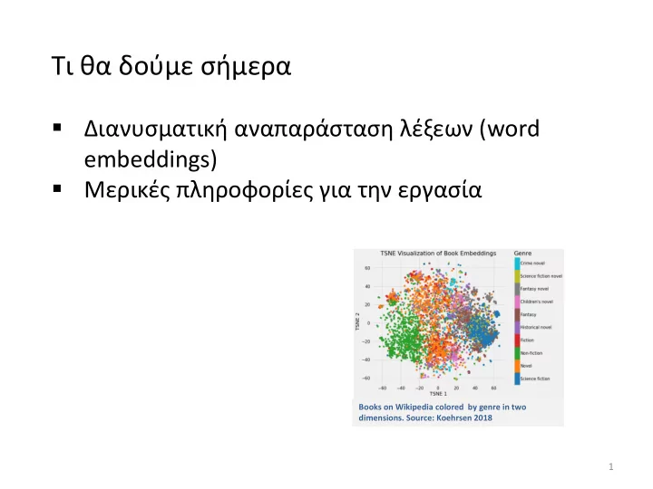
Books on Wikipedia colored by genre in two

• dimensions. Source: Koehrsen 2018

1

Τι θα δούμε σήμερα

▪ Διανυσματική αναπαράσταση λέξεων (word embeddings) ▪ Μερικές πληροφορίες για την εργασία

2

Word embeddings

3

Πρόβλημα: Διανυσματική αναπαράσταση (representation) όρων όρος διάνυσμα

embedding Στόχος: Όμοιοι όροι -> όμοια διανύσματα

4

http://suriyadeepan.github.io Παράδειγμα: 2-διάστατα embeddings

5

Apple: φρούτο και εταιρεία

https://www.analyticsvidhya.com/blog/2017/06/word-embeddings-count-word2veec/

6

Embeddings: why?

Raw Data Structured Data Learning Algorithm Model Downstream prediction task

Feature Engineering

Machine learning lifecycle

For graphs: degree, PageRank, motifs, degrees of neighbors, Pagerank of neighbors, etc For words: document

• ccurrences, k-grams. etc

For documents: length, words, etc

Classification Learning to rank Clustering

7

Embeddings: why?

Raw Data Structured Data Learning Algorithm Model Downstream prediction task

Feature Engineering

Automatically learn the features (embeddings)

Machine learning lifecycle

For graphs: degree, PageRank, motifs, degrees of neighbors, Pagerank of neighbors, etc For words: document

• ccurrences, k-grams. etc

For documents: length, words, etc

One-hot vectors

8

Έστω ότι υπάρχουν |V| διαφορετικές λέξεις (όροι) στο λεξικό μας ▪ Διατάσσουμε τις λέξεις αλφαβητικά ▪ Αναπαριστούμε κάθε λέξη με ένα R|𝑊|𝑦1 διάνυσμα που έχει παντού 0 και μόνο έναν 1 στη θέση που αντιστοιχεί στη θέση της λέξης στη διάταξη

𝟐 . . . 𝑥𝑏𝑏𝑠𝑒𝑤𝑏𝑠𝑙 = 𝟐 . . . 𝑥𝑏 = . . . 𝟐 𝑥𝑨𝑓𝑠𝑐𝑏 = 1 𝟏 . . . 𝑥𝑏𝑢 =

.. .

▪ Καμία πληροφορία για ομοιότητα ▪ Πολλές διαστάσεις

Term-Document co-occurrence matrix

9

d1 d2 d3 d4 d5 a 1 1 1 1 1 b 1 1 1 1 c 1 1 1 d 1 1 1 e 1 1 f 1

d1: a b c d2: a d a b d3: a c d e c a f d4: b e a b d5: a b d c a

Έστω ότι υπάρχουν |V| διαφορετικές λέξεις (όροι) στο λεξικό μας και |Μ| έγγραφα ▪ Κατασκευάζουμε ένα |V|xM πίνακα με τις εμφανίσεις των λέξεων στα έγγραφα ▪ Αναπαριστούμε κάθε λέξη με ένα R|Μ|𝑦1

Παράδειγμα: Word vector for c |V| = 6, |Μ| =5

Term-Document co-occurrence matrix

10

d1 d2 d3 d4 d5 a 1 2 2 1 2 b 1 1 2 1 c 1 2 1 d 1 1 1 e 1 1 f 1 Μπορούμε αντί για 0-1 να έχουμε το tf ή και το tf-idf βάρος Παράδειγμα: Word vector for c ▪ Πολλές διαστάσεις ▪ Πρόβλημα κλιμάκωσης με τον αριθμό των εγγράφων

d1: a b c d2: a d a b d3: a c d e c a f d4: b e a b d5: a b d c a

Window-based co-occurrence matrix

11

▪ Κατασκευάζουμε ένα |V|x|V| affinity-matrix για τις λέξεις: για δύο λέξεις, μετράμε τον αριθμό των φορών που αυτές δύο λέξεις εμφανίζονται μαζί σε έγγραφα ▪ Συγκεκριμένα, μετράνε τον αριθμό των φορών που κάθε λέξη εμφανίζεται μέσα σε ένα παράθυρο συγκεκριμένου μεγέθους γύρω από τη λέξη ενδιαφέροντος

Παράδειγμα: W = 1 (σε απόσταση 1) a b c d e f a 4 3 1 1 1 b 4 1 1 1 c 3 1 2 1 d 1 1 2 1 e 1 1 1 1 f 1

d1: a b c d2: a d a b d3: a c d e c a f d4: b e a b d5: a b d c a

Window-based co-occurrence matrix

12

▪ Κατασκευάζουμε ένα |V|x|V| affinity-matrix για τις λέξεις: μετράμε τον αριθμό των φορών που δυο λέξεις εμφανίζονται μέσα σε ένα παράθυρο συγκεκριμένου μεγέθους

Παράδειγμα: W = 1

d1: I enjoy flying. d2: I like NLP. d3: I like deep learning.

Λέξεις όπως apple, orange, mango, κλπ μαζί με λέξεις όπως eat, grow, cultivate, slice, κλπ και το ανάποδο ▪ Πολλές διαστάσεις

13

Θα μπορούσαμε να χρησιμοποιήσουμε μια τεχνική για να μειώσουμε τις διαστάσεις (dimensionality reduction) (πχ PCA analysis)

Singular Value Decomposition

• σ1≥ σ2≥ … ≥σn : singular values (square roots of eigenvals AAT, ATA)
• : left singular vectors (eigenvectors of AAT)
• : right singular vectors (eigenvectors of ATA)

A = U Σ VT = u1 u2 ⋯ un σ1 σ2 ⋱ σn v1 v2 ⋮ vn

[n×n] [n×n] [×n] u1,u2, ⋯ ,un v1,v2, ⋯ ,vn

▪ Cut the singular values at some index r (get the largest r such values) ▪ Get the first r columns of U to get the r-dimensional vectors

From dimension d to dimension r

Singular Value Decomposition

• r : rank of matrix A
• σ1≥ σ2≥ … ≥σr : singular values (square roots of eigenvals AAT, ATA)
• : left singular vectors (eigenvectors of AAT)
• : right singular vectors (eigenvectors of ATA)

 

                        = =

r 2 1 r 2 1 r 2 1 T

v v v σ σ σ u u u V Σ U A         

[n×r] [r×r] [r×n]

r 2 1

u , , u , u    

r 2 1

v , , v , v    

T r r r T 2 2 2 T 1 1 1 r

v u σ v u σ v u σ A        + + + =

Ar best approximation of A (Frobernius norm)

16

Αλλά ▪ Δύσκολο να ενημερώσουμε, πχ, αλλάζουν οι διαστάσεις συχνά ▪ Αραιός πίνακας ▪ Πολύ μεγάλες διαστάσεις Θα δούμε μια τεχνική που βασίζεται σε επαναληπτικές μεθόδους

word2vec

17

Basic Idea

18

• You can get a lot of value by representing a

word by means of its neighbors

• “You shall know a word by the company it

keeps”

• (J. R. Firth 1957: 11)
• One of the most successful ideas of modern

statistical NLP

government debt problems turning into banking crises as has happened in saying that Europe needs unified banking regulation to replace the hodgepodge

 These words will represent banking 

Basic idea

Define a model that aims to predict between a center word wc and context words in some window of length m in terms of word vectors P 𝑥𝑑 𝑥𝑑−𝑛, … , 𝑥𝑑−1, 𝑥𝑑+1 … , 𝑥𝑑+𝑛) Loss function 1-P that we want to minimize

20

Basic idea

Define a model that aims to predict between a center word wc and context words in some window of length m in terms of word vectors P 𝑥𝑑 𝑥𝑑−𝑛, … , 𝑥𝑑−1, 𝑥𝑑+1 … , 𝑥𝑑+𝑛) Loss function 1-P that we want to minimize Pairwise probabilities Independence assumption (bigram model) 𝑄(𝑥1, 𝑥2, …, 𝑥𝑜) = ς𝑗=2

𝑜

𝑄(𝑥𝑗|𝑥𝑗−1)

Word2Vec

22

Predict between every word and its context words

Two algorithms

• 1. Skip-grams (SG)

Predict context words given the center word

• 2. Continuous Bag of Words (CBOW)

Predict center word from a bag-of-words context Position independent (do not account for distance from center) Two training methods

• 1. Hierarchical softmax
• 2. Negative sampling

Tomas Mikolov, Ilya Sutskever, Kai Chen, Gregory S. Corrado, Jeffrey Dean: Distributed Representations of Words and Phrases and their Compositionality. NIPS 2013: 3111-3119

Note

23

N |V|

Z

𝑨𝑗

i

Each word is assigned a single N-dimensional vector Learn embedding matrix Z: each column i is the embedding 𝑨𝑗 of word i

Dimension/size

• f the embedding

|V| number of words N size of embedding m size of the window (context)

Note

24

Z

𝑨𝑗

i

𝐹𝑂𝐷 𝑗 = 𝑎 𝐽𝑗

1

i

One-hot or indicator vector, all 0s but position i 𝑃𝑜𝑓 ℎ𝑝𝑢 𝑤𝑓𝑑𝑢𝑝𝑠 𝐽𝑗

Encoder is an embedding lookup

CBOW

25

|V| number of words N size of embedding m size of the window (context)

Use a window of context words to predict the center word

Input: 2m context words Output: center word each represented as a one-hot vector

CBOW

26

Use a window of context words to predict the center word Learns two matrices (two embeddings per word, one when context,

• ne when center)

|V| Embedding of the i-th word when center word i N

W W’

N |V| i Embedding of the i-th word when context word

|V| x N context embeddings when input N x |V| center embeddings when output

CBOW

27

Use a window of context words to predict the center word

Intuition The W’-embedding of the center word should be similar to the W-embeddings of its context words

▪ For similarity, we will use cosine (dot product) ▪ We will take the average of the W-embeddings of the context word We want similarity close to one for the center word and close to 0 for all other words

CBOW

28

Given window size m 𝑦(𝑑) one hot vector for context words, y one hot vector for the center word

• 1. Input: the one hot vectors for the 2m context words

𝑦(𝑑−𝑛), …, 𝑦(𝑑−1), 𝑦(𝑑+1), …, 𝑦(𝑑+𝑛)

• 2. Compute the embeddings of the context words

𝑤𝑑−𝑛 = 𝑋𝑦(𝑑−𝑛), …, 𝑤𝑑−1 = 𝑋𝑦(𝑑−1), 𝑤𝑑+1 = 𝑋𝑦(𝑑+1), …, 𝑤𝑑+𝑛= 𝑋𝑦(𝑑+𝑛)

• 3. Average these vectors

ො 𝑤 = 𝑤𝑑−𝑛+𝑤𝑑−𝑛+1+⋯𝑤𝑑+𝑛

2𝑛

, ො 𝑤 ∈ 𝑆𝑂

• 4. Generate a score vector

z = W’ ො 𝑤 dot product, (embedding of center word), similar vectors close to each other

• 5. Turn the score vector to probabilities

ො 𝑧 = softmax(z)

We want this to be close to 1 for the center word

29

30

Exponentiate to make positive Normalize to give probability

• E.g. “The cat sat on floor”

– Window size = 2

31

the cat

• n

floor sat

32

1 … 1 …

cat

• n

1 …

Input layer Hidden layer sat Output layer

• ne-hot

vector

• ne-hot

vector Index of cat in vocabulary

33

1 … 1 …

cat

• n

1 …

Input layer Hidden layer sat Output layer

𝑋

𝑊×𝑂

𝑋

𝑊×𝑂

V-dim V-dim N-dim

𝑋′𝑂×𝑊

V-dim N will be the size of word vector We must learn W and W’

34

1 … 1 …

xcat xon

1 …

Input layer Hidden layer sat Output layer V-dim V-dim N-dim V-dim + ො 𝑤 = 𝑤𝑑𝑏𝑢 + 𝑤𝑝𝑜 2

0.1 2.4 1.6 1.8 0.5 0.9 … … … 3.2 0.5 2.6 1.4 2.9 1.5 3.6 … … … 6.1 … … … … … … … … … … … … … … … … … … … … 0.6 1.8 2.7 1.9 2.4 2.0 … … … 1.2

×

1 …

𝑋

𝑊×𝑂 𝑈

× 𝑦𝑑𝑏𝑢 = 𝑤𝑑𝑏𝑢

2.4 2.6 … … 1.8

=

35

1 … 1 …

xcat xon

1 …

Input layer Hidden layer sat Output layer V-dim V-dim N-dim V-dim + ො 𝑤 = 𝑤𝑑𝑏𝑢 + 𝑤𝑝𝑜 2

0.1 2.4 1.6 1.8 0.5 0.9 … … … 3.2 0.5 2.6 1.4 2.9 1.5 3.6 … … … 6.1 … … … … … … … … … … … … … … … … … … … … 0.6 1.8 2.7 1.9 2.4 2.0 … … … 1.2

×

1 …

𝑋

𝑊×𝑂 𝑈

× 𝑦𝑝𝑜 = 𝑤𝑝𝑜

1.8 2.9 … … 1.9

=

36

1 … 1 …

cat

• n

1 …

Input layer Hidden layer ො 𝑧sat Output layer

𝑋

𝑊×𝑂

𝑋

𝑊×𝑂

V-dim V-dim N-dim

𝑋

𝑊×𝑂 ′

× ො 𝑤 = 𝑨

V-dim N will be the size of word vector ො 𝑤

ො 𝑧 = 𝑡𝑝𝑔𝑢𝑛𝑏𝑦(𝑨)

37

1 … 1 …

cat

• n

1 …

Input layer Hidden layer ො 𝑧sat Output layer

𝑋

𝑊×𝑂

𝑋

𝑊×𝑂

V-dim V-dim N-dim

𝑋

𝑊×𝑂 ′

× ො 𝑤 = 𝑨 ො 𝑧 = 𝑡𝑝𝑔𝑢𝑛𝑏𝑦(𝑨)

V-dim N will be the size of word vector ො 𝑤

0.01 0.02 0.00 0.02 0.01 0.02 0.01 0.7 … 0.00

ො 𝑧 We would prefer ො 𝑧 close to ො 𝑧𝑡𝑏𝑢

38

1 … 1 …

xcat xon

1 …

Input layer Hidden layer sat Output layer V-dim V-dim N-dim V-dim

𝑋

𝑊×𝑂

𝑋

𝑊×𝑂

0.1 2.4 1.6 1.8 0.5 0.9 … … … 3.2 0.5 2.6 1.4 2.9 1.5 3.6 … … … 6.1 … … … … … … … … … … … … … … … … … … … … 0.6 1.8 2.7 1.9 2.4 2.0 … … … 1.2

𝑋

𝑊×𝑂 𝑈

Contain word’s vectors

𝑋

𝑊×𝑂 ′

We can consider either W (context) or W’ (center) as the word’s representation. Or even take the average.

Skipgram

39

Given the center word, predict (or, generate) the context words Input: center word Output: 2m context word each represented as a one-hot vectors Learn two matrices W: N x |V|, input matrix, word representation as center word W’: |V| x N, output matrix, word representation as context word

40

Skipgram

41

𝑧(𝑘) one hot vector for context words

• 1. Input: one hot vector of the center word

𝑦

• 2. Get the embedding of the center word

𝑤𝑑 = 𝑋 𝑦

• 3. Generate a score vector for each context word

z = W’ 𝑤𝑑

• 5. Turn the score vector into probabilities

ො 𝑧 = softmax(z) We want this to be close to 1 for the context words

Given the center word, predict (or, generate) the context words

42

Skipgram

43

• For each word t = 1 … T, predict surrounding words in a

window of “radius” m of every word.

• Objective function: Maximize the probability of any

context word given the current center word: where θ represents all variables we will optimize

44

An example

Word2Vec

45

Predict between every word and its context words

Two algorithms

• 1. Skip-grams (SG)

Predict context words given the center word

• 2. Continuous Bag of Words (CBOW)

Predict center word from a bag-of-words context Position independent (do not account for distance from center) Two training methods

• 1. Hierarchical softmax
• 2. Negative sampling

Tomas Mikolov, Ilya Sutskever, Kai Chen, Gregory S. Corrado, Jeffrey Dean: Distributed Representations of Words and Phrases and their Compositionality. NIPS 2013: 3111-3119

Training methods: hierarchical softmax

46

Στόχος: Αντί να μάθουμε ένα διάνυσμα ανά λέξη, δηλαδή |V| διανύσματα, να μάθουμε 𝑚𝑝𝑕2 𝑊 διανύσματα Πως; Ένα δυαδικό δέντρο Ένα φύλλο ανά λέξη Μαθαίνουμε την αναπαράσταση των εσωτερικών κόμβων Αναπαράσταση λέξης: concat των αναπαραστάσεων των κόμβων στο μονοπάτι από τη ρίζα στη λέξη

Training methods: negative sampling

47

Στόχος: Να βελτιώσουμε την ποιότητα των αναπαραστάσεων με χρήση αρνητικών δειγμάτων ▪ Για κάθε ένα θετικό, Κ αρνητικά δείγματα ▪ Χρήση unigram μοντέλου για να τα κατασκευάσουμε

48

These representations are very good at encoding similarity and dimensions of similarity!

• Analogies testing dimensions of similarity can

be solved quite well just by doing vector subtraction in the embedding space

Syntactically – xapple − xapples ≈ xcar − xcars ≈ xfamily − xfamilies – Similarly for verb and adjective morphological forms Semantically – xshirt − xclothing ≈ xchair − xfurniture – xking − xman ≈ xqueen − xwoman

49

king man woman

Test for linear relationships, examined by Mikolov et al.

man woman [ 0.20 0.20 ] [ 0.60 0.30 ] king [ 0.30 0.70 ] [ 0.70 0.80 ]

− + +

man:woman :: king:?

a:b :: c:?

queen

50

51

▪ Στην εργασία, σας ζητείτε να χρησιμοποιείστε word embeddings

▪ Πρέπει να επιλέξετε πως ▪ Θα αξιολογηθεί και η καταλληλότητα/πρωτοτυπία/χρησιμότητα

▪ Στη συνέχεις θα δούμε ▪ pretrained embeddings ▪ μερικές εφαρμογές

52

Σύντομη περιγραφή της εργασίας

• 1. Θα συλλέξετε έναν αριθμό από Wikipedia άρθρα

Αυτή θα είναι η συλλογή σας.

• 2. Θα υλοποιήσετε ένα σύστημα αναζήτησης (ΣΑΠ) αυτών

των άρθρων: Ο χρήστης θα δίνει μία ή περισσότερες λέξεις κλειδιά και το σύστημα θα επιστρέφει τα πιο συναφή άρθρα σε διάταξη με βάση τη συνάφεια τους στην ερώτηση Για να υλοποιήσετε το σύστημα θα χρησιμοποιείστε τη

• Lucene. Περισσότερα την επόμενη ώρα.

Global vs. local embedding

[Diaz 2016]

Πάνω σε ποια συλλογή (corpus) φτιάχνουμε τα embeddings; Προτάσεις από ποια κείμενα θα χρησιμοποιήσουμε;

54

https://code.google.com/archive/p/word2vec/

• 1. Train and create embeddings based on a local collection

Python implementation in gensim https://radimrehurek.com/gensim/models/word2vec.html

• 2. Use pretrained embeddings

https://fasttext.cc/docs/en/crawl-vectors.html Pretrained embeddings for 157 languages Google https://www.tensorflow.org/tutorials/text/word_embeddings Tensorflow

55

Finding the degree of similarity between two words.

model.similarity('woman','man') 0.73723527

Finding odd one out.

model.doesnt_match('breakfast cereal dinner lunch';.split()) 'cereal'

Amazing things like woman+king-man =queen

model.most_similar(positive=['woman','king'],negative=['man'],top n=1) queen: 0.508

Probability of a text under the model

model.score(['The fox jumped over the lazy dog'.split()]) 0.21

ανεκτική ανάκτηση: (1) επέκταση ερωτήματος ή/και (2) context-dependent διόρθωση λάθους, όπου θα μπορούσαμε να χρησιμοποιήσουμε και το query log και γενικά query suggestions

56

bilingual embedding with chinese in green and english in yellow

Improve language translation

By aligning the word embeddings for the two languages

57

Είδαμε διάταξη με 𝑟𝑈𝑒 ෍

𝑥∈𝑟

𝑥𝑒′

Όπου w το embedding των λέξεων της ερώτησης και d’ το embedding του εγγράφου (π.χ., το μέσο των embedding των λέξεων του εγγράφου) ▪ Στόχος: Σχέση ερώτησης με το όλο το περιεχόμενο του εγγράφου ▪ Input (center word) embedding ή output (context) word embedding; in- query, out-document ▪ Σε συνδυασμό με άλλα κριτήρια

Χρήση στη διάταξη των εγγράφων του αποτελέσματος μιας ερώτησης

Μπορούμε να χρησιμοποιήσουμε embeddings; Πολλές εναλλακτικές, για παράδειγμα (aboutness)

End of lecture

58

Χρησιμοποιήθηκε υλικό από ▪ CS276: Information Retrieval and Web Search, Christopher Manning and Pandu Nayak, Lecture 14: Distributed Word Representations for Information Retrieval ▪ https://www.analyticsvidhya.com/blog/2017/06/word-embeddings-count-word2veec/ Μια περιγραφή του skipgram: Chris McCormick http://mccormickml.com/2016/04/19/word2vec-tutorial-the-skip-gram-model/ Δείτε και το https://www.analyticsvidhya.com/blog/2017/06/word-embeddings-count-word2veec/

Extra slides

Hierarchical softmax and negative sampling

59

Hierarchical softmax

60

Instead of learning O(|V|) vectors, learn O(log(|V|) vectors How? ▪ Build a binary tree with leaves the words, and learn one vector for each internal node. ▪ The value for each word w is the product of the values of the internal nodes in the path from the root to w.

61

The probability of a word being the context word is defined as: where:

– 𝑜 𝑥, 𝑘 – is the j-th node on the path from the root to w. – 𝑀 𝑥 – is the length of the path from root to w. – 𝑑ℎ(𝑜) – is the left child of node n. – 𝑦 = { 1 𝑗𝑔 𝑦 𝑗𝑡 𝑢𝑠𝑣𝑓 −1 𝑝𝑢ℎ𝑓𝑠𝑥𝑗𝑡𝑓 – 𝜏 𝑦 =

1 1+𝑓−𝑦

𝑞 𝑑 𝑥 = ෑ

𝑘=1 𝑀 𝑥 −1

𝜏( 𝑜 𝑑, 𝑘 + 1 = 𝑑ℎ(𝑜(𝑥, 𝑘)) ∙ 𝑤𝑜(𝑑,𝑘)

𝑈𝑤𝑥)

returns 1 if the path goes left,

• 1 if it goes right

n w, 1 = root n w, L w = parent of w L w2 = 3

compares the similarity of the input vector 𝑤𝑥 to each internal node vector

62

Suppose we want to compute the probability of w2 being the output word.

• The probabilities of going right/left in a node n are:

– 𝑞 𝑜, 𝑚𝑓𝑔𝑢 = 𝜏 𝑤𝑜

𝑈𝑤𝑥

– 𝑞 𝑜, 𝑠𝑗𝑕ℎ𝑢 = 1 − 𝜏 𝑤𝑜

𝑈𝑤𝑥 = 𝜏 −𝑤𝑜 𝑈𝑤𝑥

𝑞 𝑥2 = 𝑑 = 𝑞 𝑜 𝑥2, 1 , 𝑚𝑓𝑔𝑢 ∙ 𝑞 𝑜 𝑥2, 2 , 𝑚𝑓𝑔𝑢 ∙ 𝑞 𝑜 𝑥2, 3 , 𝑠𝑗𝑕ℎ𝑢 = 𝜏 𝑤𝑜 𝑥2,1

𝑈𝑤𝑥 ∙ 𝜏 𝑤𝑜 𝑥2,2 𝑈𝑤𝑥 ∙ 𝜏 −𝑤𝑜 𝑥2,3 𝑈𝑤𝑥

Complexity improved even further using a Huffman tree: ▪ Designed to compress binary code of a given text. ▪ A full binary suffix tree that guarantees a minimal average weighted path length when some words are frequently used.

Negative Sampling

63

▪ For each positive example we draw K negative examples. ▪ The negative examples are drawn according to the unigram distribution of the data

64

p 𝐸 = 1|𝑥, 𝑑 is the probability that 𝑥, 𝑑 ∈ 𝐸. p 𝐸 = 0|𝑥, 𝑑 = 1 − p 𝐸 = 1|𝑥, 𝑑 is the probability that (𝑥, 𝑑) ∉ D. For negative samples: 𝑞(𝐸 = 1|𝑥, 𝑑) must be low ⇒ 𝑞(𝐸 = 0|𝑥, 𝑑) will be high.

For one sample:

Extra slides

Neural nets (from our graduate class with P. Tsaparas)

65

INTRODUCTION TO NEURAL NETWORKS

(Thanks to Philipp Koehn for the material borrowed from his slides)

66

Classification

• Classification is the task of learning a target function f that maps attribute set x

to one of the predefined class labels y

Tid Refund Marital Status Taxable Income Cheat 1 Yes Single 125K No 2 No Married 100K No 3 No Single 70K No 4 Yes Married 120K No 5 No Divorced 95K Yes 6 No Married 60K No 7 Yes Divorced 220K No 8 No Single 85K Yes 9 No Married 75K No 10 No Single 90K Yes

One of the attributes is the class attribute In this case: Cheat Two class labels (or classes): Yes (1), No (0)

Illustrating Classification Task

Apply Model

Induction Deduction

Learn Model

Model

Tid Attrib1 Attrib2 Attrib3 Class 1 Yes Large 125K No 2 No Medium 100K No 3 No Small 70K No 4 Yes Medium 120K No 5 No Large 95K Yes 6 No Medium 60K No 7 Yes Large 220K No 8 No Small 85K Yes 9 No Medium 75K No 10 No Small 90K Yes

Tid Attrib1 Attrib2 Attrib3 Class 11 No Small 55K ? 12 Yes Medium 80K ? 13 Yes Large 110K ? 14 No Small 95K ? 15 No Large 67K ?

Test Set Learning algorithm Training Set

Example of a Model

Tid Refund Marital Status Taxable Income Cheat 1 Yes Single 125K No 2 No Married 100K No 3 No Single 70K No 4 Yes Married 120K No 5 No Divorced 95K Yes 6 No Married 60K No 7 Yes Divorced 220K No 8 No Single 85K Yes 9 No Married 75K No 10 No Single 90K Yes

Refund MarSt TaxInc YES NO NO NO Yes No Married Single, Divorced < 80K > 80K

Training Data Model: Decision Tree

Classification in Networks

• There are various problems in network analysis that

can be mapped to a classification problem:

– Link prediction: Predict 0/1 for missing edges, whether they will appear or not in the future. – Node classification: Classify nodes as democrat- republican/spammers-legitimate/other categories

• Use node features but also neighborhood and structural features
• Label propagation

– Edge classification: Classify edges according to type (professional/family relationships), or according to strength. – More…

• Recently all of this is done using Neural Networks.

70

Linear Classification

• A simple model for classification is to take a linear

combination of the feature values and compute a score.

• Input: Feature vector 𝒚 = (𝑦1, … , 𝑦𝑜)
• Model: Weights 𝒙 = (𝑥1, … , 𝑥𝑜)
• Output: 𝑡𝑑𝑝𝑠𝑓 𝒙, 𝒚 = σ𝑗 𝑥𝑗𝑦𝑗
• Make a decision depending on the output score.

– E.g.: Decide “Yes” if 𝑡𝑑𝑝𝑠𝑓 𝒙, 𝒚 > 0 and “No” if 𝑡𝑑𝑝𝑠𝑓 𝒙, 𝒚 < 0

71

Linear Classification

• We can represent this as a network

72

Input nodes correspond to features 𝑦1 𝑦3 𝑦4 𝑦5 𝑦2 𝑥1 𝑥2 𝑥3 𝑥4 𝑥5 Edges correspond to weights 𝑡𝑑𝑝𝑠𝑓(𝒙, 𝒚) “Output” node with incoming edges computes the score

Linear models

• Linear models partition the space according to a

hyperplane

• But they cannot model everything

73

Multiple layers

• We can add more layers:

– Each arrow has a weight – Nodes compute scores from incoming edges and give input to

• utgoing edges

74

Did we gain anything?

Non-linearity

• Instead of computing a linear combination

𝑡𝑑𝑝𝑠𝑓 𝒙, 𝒚 = ෍

𝑗

𝑥𝑗𝑦𝑗

• Apply a non-linear function on top:

𝑡𝑑𝑝𝑠𝑓 𝒙, 𝒚 = 𝑕 ෍

𝑗

𝑥𝑗𝑦𝑗

• Popular functions:

75

These functions play the role of a soft “switch” (threshold function)

Side note

• Logistic regression classifier:

– Single layer with a logistic function

76

Deep learning

• Networks with multiple layers
• Each layer can be thought of as a processing step
• Multiple layers allow for the computation of more

complex functions

77

Example

• A network that implements XOR

78

Hidden node ℎ0 is OR Bias term Hidden node ℎ1 is AND Output node ℎ1 − ℎ0

Error

• The computed value is 0.76 but the correct value

is 1

– There is an error in the computation – How do we set the weights so as to minimize this error?

79

Gradient Descent

• The error is a function of the weights
• We want to find the weights that minimize the

error

• Compute gradient: gives the direction to the

minimum

• Adjust weights, moving at the direction of the

gradient.

80

Gradient Descent

81

Gradient Descent

82

Backpropagation

• How can we compute the gradients?

Backpropagation!

• Main idea:

– Start from the final layer: compute the gradients for the weights of the final layer. – Use these gradients to compute the gradients of previous layers using the chain rule – Propagate the error backwards

• Backpropagation essentially is an application of

the chain rule for differentiation.

83

84

𝑦1 𝑦2 ℎ2 𝑧2 𝑧1 ℎ1 𝑏11 𝑏22 𝑏21 𝑏12 𝑐11 𝑐22 𝑐21 𝑐12 Error: 𝐹 = 𝑧 − 𝑢 2 = 𝑧1 − 𝑢1 2 + 𝑧2 − 𝑢2 2 Notation: Activation function: 𝑕 𝑡𝑧1 = 𝑐11ℎ1 + 𝑐12ℎ2 , 𝑧1 = 𝑕 𝑡𝑧1 𝑡𝑧2 = 𝑐21ℎ1 + 𝑐22ℎ2 , 𝑧2 = 𝑕(𝑡𝑧2) 𝑡ℎ1 = 𝑏11𝑦1 + 𝑏12𝑦2 , ℎ1 = 𝑕(𝑡ℎ1) 𝑡ℎ2 = 𝑏21𝑦1 + 𝑏22𝑦2 , ℎ2 = 𝑕(𝑡ℎ2) 𝜖𝐹 𝜖𝑐11 = 𝜖𝐹 𝜖𝑡𝑧1 𝜖𝑡𝑧1 𝜖𝑐11 = 𝜀𝑧1ℎ1 𝜖𝐹 𝜖𝑏11 = 𝜖𝐹 𝜖𝑡ℎ1 𝜖𝑡ℎ1 𝜖𝑏11 = 𝜀ℎ1𝑦1 𝜀𝑧1= 𝜖𝐹

𝜖𝑡𝑧1= 𝜖𝐹 𝜖𝑧1 𝜖𝑧1 𝜖𝑡𝑧1 = 2 𝑧1 − 𝑢1 𝑕′(𝑡𝑧1)

𝜖𝐹 𝜖𝑐21 = 𝜀𝑧2ℎ1 𝜀𝑧2= 𝜖𝐹

𝜖𝑡𝑧2 = 2 𝑧2 − 𝑢2 𝑕′(𝑡𝑧2)

𝜖𝐹 𝜖𝑐12 = 𝜀𝑧1ℎ2 𝜖𝐹 𝜖𝑐22 = 𝜀𝑧2ℎ2 𝜀ℎ1 = 𝜖𝐹 𝜖𝑡ℎ1 = 𝜖𝐹 𝜖ℎ1 𝜖ℎ1 𝜖𝑡ℎ1 = 𝜖𝐹 𝜖𝑡𝑧1 𝜖𝑡𝑧1 𝜖ℎ1 + 𝜖𝐹 𝜖𝑡𝑧2 𝜖𝑡𝑧2 𝜖ℎ1 𝑕′ 𝑡ℎ1 = 𝜀𝑧1𝑐11 + 𝜀𝑧2𝑐21 𝑕′(𝑡ℎ1) 𝜀ℎ2 = 𝜀𝑧1𝑐12 + 𝜀𝑧2𝑐22 𝑕′(𝑡ℎ2) 𝜖𝐹 𝜖𝑏22 = 𝜖𝐹 𝜖𝑡ℎ2 𝜖𝑡ℎ2 𝜖𝑏22 = 𝜀ℎ2𝑦2 𝜖𝐹 𝜖𝑏21 = 𝜀ℎ1𝑦2 𝜖𝐹 𝜖𝑏12 = 𝜀ℎ2𝑦1

Backpropagation

85

𝑦𝑘 ℎ𝑗 𝑏𝑗𝑘 𝑧1 𝑧𝑙 𝑧𝑜 𝑐𝑙𝑗 𝑐1𝑗 𝑐𝑜𝑗 𝑡𝑧1 𝑡𝑧𝑙 𝑡𝑧𝑜 𝜀𝑧1 = 𝜖𝐹 𝜖𝑡𝑧1 𝜀𝑧𝑙 = 𝜖𝐹 𝜖𝑡𝑧𝑙 𝜀𝑧𝑜 = 𝜖𝐹 𝜖𝑡𝑧𝑜 𝜖𝐹 𝜖𝑏𝑗𝑘 = ෍

𝑙=1 𝑜

𝜀𝑧𝑙𝑐𝑙𝑗 𝑕′ 𝑡ℎ𝑗 𝑦𝑘 𝑡ℎ𝑗 For the sigmoid function: 𝑕 𝑦 = 1 1 + 𝑓−𝑦 The derivative is: 𝑕′ 𝑦 = 𝑕(𝑦)(1 − 𝑕 𝑦 ) This makes it easy to compute it. We have: 𝑕′ 𝑡ℎ𝑗 = ℎ𝑗(1 − ℎ𝑗)

Stochastic gradient descent

• Ideally the loss should be the average loss over all

training data.

• We would need to compute the loss for all

training data every time we update the gradients.

– However, this is expensive.

• Stochastic gradient descent: Consider one input

point at the time. Each point is considered only

• nce.
• Intermediate solution: Use mini-batches of data

points.

86

87

End of extra slides