Why team theory and distributed control? Many control tasks are - - PDF document

SLIDE 1

1 Linear quadratic theory for distributed control — From telescopes to vehicle formations

Anders Rantzer

Automatic Control LTH, Lund University

Why team theory and distributed control?

Many control tasks are naturally distributed, i.e. many controllers are supposed to work together in a team.

◮ Vehicle dynamics ◮ Vehicle formations ◮ Electrical power network ◮ Power control in cell phone

network

G1 G3 G5 G8 G9 G11 G12 G15 G13 G10 G16 G14 G7 G2 G4 G6

The EURO 50 Telescope Large Deformable Mirror Control of Deformable Mirror

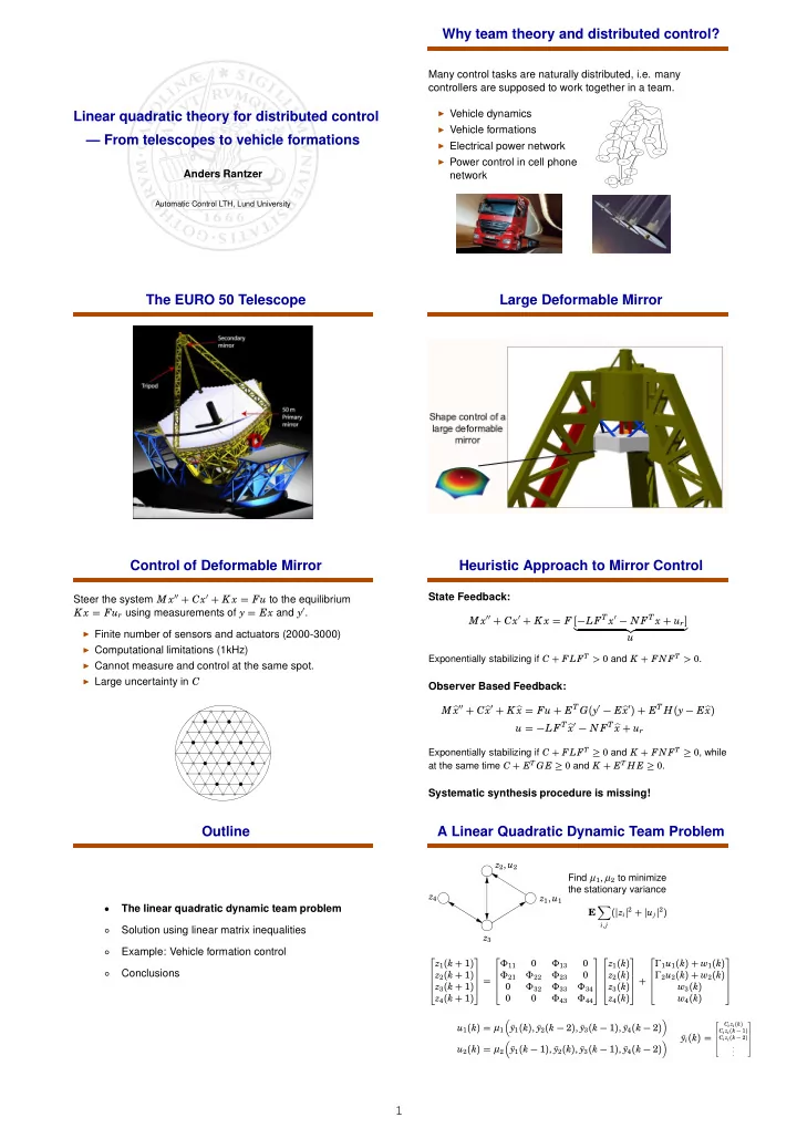
Steer the system M x′′ + Cx′ + K x = Fu to the equilibrium K x = Fur using measurements of y = Ex and y′.

◮ Finite number of sensors and actuators (2000-3000) ◮ Computational limitations (1kHz) ◮ Cannot measure and control at the same spot. ◮ Large uncertainty in C

Heuristic Approach to Mirror Control

State Feedback: M x′′ + Cx′ + K x = F [−LFT x′ − N FT x + ur]

• u

Exponentially stabilizing if C + FLFT > 0 and K + FNFT > 0.

Observer Based Feedback: M x′′ + C x′ + K x = Fu + ET G(y′ − E x′) + ET H(y − E x) u = −LFT x′ − N FT x + ur

Exponentially stabilizing if C + FLFT ≥ 0 and K + FNFT ≥ 0, while at the same time C + ET GE ≥ 0 and K + ET H E ≥ 0.

Systematic synthesis procedure is missing!

Outline

• The linear quadratic dynamic team problem

○ Solution using linear matrix inequalities ○ Example: Vehicle formation control ○ Conclusions

A Linear Quadratic Dynamic Team Problem

z1, u1 z2, u2 z3 z4 Find µ1, µ2 to minimize the stationary variance E

• i,j

(zi2 + uj2)     z1(k + 1) z2(k + 1) z3(k + 1) z4(k + 1)     =     Φ11 Φ13 Φ21 Φ22 Φ23 Φ32 Φ33 Φ34 Φ43 Φ44         z1(k) z2(k) z3(k) z4(k)     +     Γ1u1(k) + w1(k) Γ2u2(k) + w2(k) w3(k) w4(k)     u1(k) = µ1

• ¯

y1(k), ¯ y2(k − 2), ¯ y3(k − 1), ¯ y4(k − 2)

• u2(k) = µ2
• ¯

y1(k − 1), ¯ y2(k), ¯ y3(k − 1), ¯ y4(k − 2)

• ¯

yi(k) =

2 6 6 6 6 4 Ci zi(k) Ci zi(k − 1) Ci zi(k − 2) . . . 3 7 7 7 7 5

SLIDE 2

2 The Witsenhausen counterexample

x1 = x0 + µ1(x0) x2 = x1 − µ2(x1 + v) Minimize E [k2(µ1(x0))2 + (x2)2] when x0 and v are given Gaussian variables. The best controllers are not linear. The output of the first controller appears as input of the second. Hence there is an incentive for the first controller to “signal” its information to the second controller. [ Radner (1962) Team decision problems ] [ Witsenhausen (1968) A counterexample in stochastic control ]

Finite time optimal LQ optimal control

[Yu-Chi Ho and K’ai-Ching Chu (1972)]: “If a decision-makers action affects our information, then knowing what he knows will yield linear optimal solutions” z1, u1 z2, u2 z3 z4 Find µ1, µ2 to minimize E

T

• k=0
• i,j

(zi(k)2 + uj(k)2)     z1(k + 1) z2(k + 1) z3(k + 1) z4(k + 1)     =     Φ11 Φ13 Φ21 Φ22 Φ23 Φ32 Φ33 Φ34 Φ43 Φ44         z1(k) z2(k) z3(k) z4(k)     +     Γ1u1(k) + w1(k) Γ2u2(k) + w2(k) w3(k) w4(k)     u1(k) = µ1

• ¯

y1(k), ¯ y2(k − 2), ¯ y3(k − 1), ¯ y4(k − 2)

• u2(k) = µ2
• ¯

y1(k − 1), ¯ y2(k), ¯ y3(k − 1), ¯ y4(k − 2)

• ¯

yi(k) =

2 6 6 6 6 4 Ci zi(k) Ci zi(k − 1) Ci zi(k − 2) . . . 3 7 7 7 7 5

Convexity in distributed control

A recent observation by [Bamieh, Voulgaris (2002)] and [Rotkowitz, Lall (2002)]: The signaling incentive disappears and the distributed control synthesis problem becomes convex provided that communication links propagate information faster than the process does.

Quadratic Invariance

[Rotkowitz, Lall (2002)]: Let S be a linear space. Original problem: MinimizeK∈S T11 + T12K(I − T22K)−1T21 Modified problem: MinimizeQ∈S T11 + T12QT21 Conditions for equivalence between the two:

The two are equivalent if S is quadratically invariant under T22, i.e. K T22K ∈ S for all K ∈ S This holds even for nonlinear operators if K1T22K2 ∈ S for all K1, K2 ∈ S

Outline

○ The linear quadratic dynamic team problem

• Solution using linear matrix inequalities

○ Example: Vehicle formation control ○ Conclusions

Standard linear quadratic optimal control

Find u = Lx to minimize E(xT Qxxx + uT Quuu + 2xT Qxuu) when x+ = Ax + Bu + w EwwT = I

Solution by convex optimization: Minimize trace

• Qxx

Qxu Qux Quu Xxx Xxu Xux Xuu

• subject to

Xxx =

• A

B I

• 

 Xxx Xxu Xux Xuu I  

• >0

  AT BT I  

Then put u = Xux X −1

xx x

Control with disturbance measurements

Find u = Lx to minimize E(xT Qxxx + uT Quuu + 2xT Qxuu) when x+ = Ax + Bu + w EwwT = I

Solution by convex optimization: Minimize trace

• Qxx

Qxu Qux Quu Xxx Xxu Xux Xuu

• subject to

Xxx =

• A

B I

• 

 Xxx Xxu Xux Xuu Xuw Xwu I  

• >0

  AT BT I  

Then put u = Xux X −1

xx x + Xuww

With one-step delay information pattern

Find u = Lx +

• M1

M2

• w to minimize E(xT Qxxx + uT Quuu + 2xT Qxuu)

where x+ = Ax + Bu + w EwwT = I

Solution by convex optimization: Minimize trace

• Qxx

Qxu Qux Quu Xxx Xxu Xux Xuu

• subject to

Xxx =

• A

B I

• 

 Xxx Xxu Xux Xuu Xuw Xwu I  

• >0

  AT BT I   Xuw = X T

wu =

M1

M2

• Then put u = Xux X −1

xx x + Xuww

SLIDE 3

3 Lagrange multiplier method works here!

Already in Yakubovich’s SCL-92 paper, a new result by Megretski and Trail was used to prove that Minimize φ0(u) subject to φ1(u) = 0, . . . ,φn(u) = 0 is equivalent to Minimize φ0(u) + λ1φ1(u) + ⋅ ⋅ ⋅ + λnφn(u) for some value of λ1, . . . ,λn. Hence covariance constraints can be used for distributed

• control. Separation holds because the second problem is
• rdinary LQG!

Theorem 1

The following statements are equivalent for the system z(t + 1) = Φz(t) + Γ[u(t) + w(t)] (1) (i) There exist feedback laws ui(t) = µi

• ¯

z1(t − di1), . . ., ¯ zJ(t − diJ)

• that together with (1) have a stationary zero mean

solution satisfying E Cz + Du2 ≤ γ . (ii) There exists a feedback law u(k) = µ(x) that together with (1) has a stationary zero mean solution satisfying E Cz + Du2 ≤ γ E ui(k)wj(k − l) = 0 for 1 ≤ j ≤ J and 1 ≤ l ≤ dij.

Outline

○ The linear quadratic dynamic team problem ○ Solution using linear matrix inequalities

• Example: Vehicle formation control

○ Conclusions

A vehicle formation

x1 x2 x3 x4 x5 The objective is to minimize E 4

i=1 xi+1 − xi2.

Each vehicle obeys the independent dynamics zi(k + 1) = zi(k) + ui(k) + wi(k)

A vehicle formation

No communication: x1 x2 x3 x4 x5 E x1 − x22 = 3.40 E x3 − x42 = 3.40 E x2 − x32 = 3.40 E x4 − x52 = 3.40

A vehicle formation

No communication: x1 x2 x3 x4 x5 E x1 − x22 = 3.40 E x3 − x42 = 3.40 E x2 − x32 = 3.40 E x4 − x52 = 3.40 Full state information everywhere: E x1 − x22 = 3.13 E x3 − x42 = 3.16 E x2 − x32 = 3.16 E x4 − x52 = 3.13

A vehicle formation

x1 x2 x3 x4 x5 E x1 − x22 = 3.40 E x3 − x42 = 3.40 E x2 − x32 = 3.40 E x4 − x52 = 3.40 E x1 − x22 = 3.13 E x3 − x42 = 3.16 E x2 − x32 = 3.16 E x4 − x52 = 3.13 E x1 − x22 = 3.30 E x3 − x42 = 3.33 E x2 − x32 = 3.32 E x4 − x52 = 3.25

Outline

○ The linear quadratic dynamic team problem ○ Solution using linear matrix inequalities ○ Example: Vehicle formation control

• Conclusions

SLIDE 4

4 Conclusions

◮ A large class of LQ problems previously overlooked ◮ Communication must be faster than process dynamics ◮ Solutions in terms of linear matrix inequalities ◮ Optimal estimates in sensor networks

Research needs

◮ Distributed synthesis procedure ◮ Utilize graph structure for efficient implementation ◮ Nonlinear versions ◮ Information channels with limited capacity

Inspiration during sabbatical at Caltech

◮ Spatially invariant systems

(Bamieh, Paganini, Dahleh)

◮ Distributed control using dissipativity

(Langbort, Chandra, d’Andrea)

◮ The saddle point algorithm

(Arrow, Hurwitz, Uzawa)

◮ Network congestion control

(Kelly, Paganini, Doyle, Low, ...)

◮ Stability of Kuramoto’s coupled nonlinear oscillators

(Jadbabaie, Barahona, Motee)

◮ Distributed average computation

(Xiao, Boyd) Thanks for suggestions by Peter Alriksson, Ather Gattami Vijay Gupta, Cedrik Langbort, Pablo Parrilo, Jeff Shamma

More on distributed control at this MTNS

Thursday 17:25-17:50 Distributed Stochastic Control: A Team Theoretic Approach Ather Gattami Friday 12:05-12:30 Distributed Kalman Filtering Using Weighted Averaging Peter Alriksson and Anders Rantzer