Why probability in robotics? n Often state of robot and state of its - PDF document

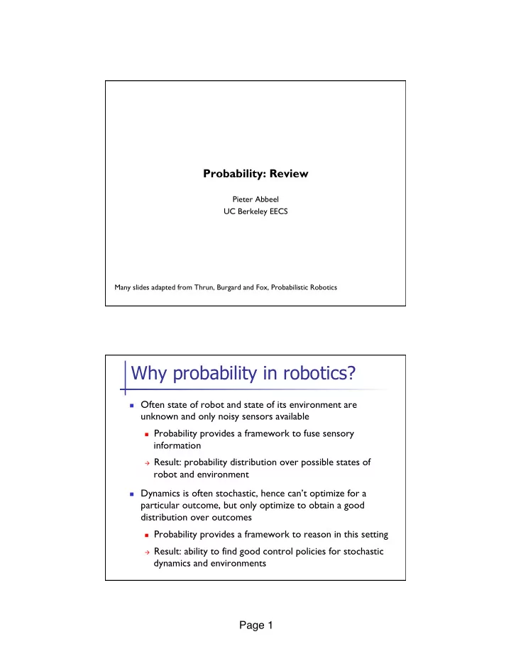
Probability: Review Pieter Abbeel UC Berkeley EECS Many slides adapted from Thrun, Burgard and Fox, Probabilistic Robotics Why probability in robotics? n Often state of robot and state of its environment are unknown and only noisy sensors available n Probability provides a framework to fuse sensory information à Result: probability distribution over possible states of robot and environment n Dynamics is often stochastic, hence can’t optimize for a particular outcome, but only optimize to obtain a good distribution over outcomes n Probability provides a framework to reason in this setting à Result: ability to find good control policies for stochastic dynamics and environments Page 1 �

Example 1: Helicopter n State: position, orientation, velocity, angular rate n Sensors: n GPS : noisy estimate of position (sometimes also velocity) n Inertial sensing unit: noisy measurements from 3-axis gyro [=angular rate sensor], (i) (ii) 3-axis accelerometer [=measures acceleration + gravity; e.g., measures (0,0,0) in free-fall], (iii) 3-axis magnetometer n Dynamics: n Noise from: wind, unmodeled dynamics in engine, servos, blades Example 2: Mobile robot inside building n State: position and heading n Sensors: n Odometry (=sensing motion of actuators): e.g., wheel encoders n Laser range finder: n Measures time of flight of a laser beam between departure and return n Return is typically happening when hitting a surface that reflects the beam back to where it came from n Dynamics: n Noise from: wheel slippage, unmodeled variation in floor Page 2 �

Axioms of Probability Theory 0 Pr( A ) 1 ≤ ≤ n n Pr( ! ) = 1 Pr( ! ) = 0 Pr( A ! B ) = Pr( A ) + Pr( B ) " Pr( A # B ) n Pr (A) denotes probability that the outcome ω is an element of the set of possible outcomes A . A is often called an event. Same for B. Ω is the set of all possible outcomes. ϕ is the empty set. 5 A Closer Look at Axiom 3 Pr( A ! B ) = Pr( A ) + Pr( B ) " Pr( A # B ) ! A B A ! B 6 Page 3 �

Using the Axioms Pr( A ! ( " \ A )) = Pr( A ) + Pr( " \ A ) # Pr( A $ ( " \ A )) Pr( " ) Pr( A ) + Pr( " \ A ) # Pr( ! ) = 1 Pr( A ) + Pr( " \ A ) # 0 = Pr( " \ A ) 1 # Pr( A ) = 7 Discrete Random Variables ! x 2 x 3 x 1 x 4 n X denotes a random variable. n X can take on a countable number of values in {x 1 , x 2 , …, x n }. n P(X=x i ) , or P(x i ) , is the probability that the random variable X takes on value x i . n P( ) is called probability mass function. . n E.g., X models the outcome of a coin flip, x 1 = head, x 2 = tail, P( x 1 ) = 0.5 , P( x 2 ) = 0.5 8 Page 4 �

Continuous Random Variables n X takes on values in the continuum. n p(X=x) , or p(x) , is a probability density function. b Pr( x ( a , b )) p ( x ) dx ∈ = ∫ a p(x) n E.g. x 9 Joint and Conditional Probability n P(X=x and Y=y) = P(x,y) n If X and Y are independent then P(x,y) = P(x) P(y) n P(x | y) is the probability of x given y P(x | y) = P(x,y) / P(y) P(x,y) = P(x | y) P(y) n If X and Y are independent then P(x | y) = P(x) n Same for probability densities, just P à p 10 Page 5 �

Law of Total Probability, Marginals Discrete case Continuous case P ( x ) 1 ∑ p ( x ) dx = 1 = ∫ x P ( x ) P ( x , y ) ∑ p ( x ) p ( x , y ) dy = = ∫ y P ( x ) P ( x | y ) P ( y ) ∑ p ( x ) p ( x | y ) p ( y ) dy = = ∫ y 11 Bayes Formula P ( x , y ) P ( x | y ) P ( y ) P ( y | x ) P ( x ) = = ⇒ P ( y | x ) P ( x ) likelihood prior ⋅ P ( x y ) = = P ( y ) evidence 12 Page 6 �

Normalization P ( y | x ) P ( x ) P ( x y ) P ( y | x ) P ( x ) = = η P ( y ) 1 1 P ( y ) − η = = P ( y | x ) P ( x ) ∑ x Algorithm: x : aux P ( y | x ) P ( x ) ∀ = x | y 1 η = aux ∑ x | y x x : P ( x | y ) aux ∀ = η x | y 13 Conditioning n Law of total probability: P ( x ) P ( x , z ) dz = ∫ P ( x ) P ( x | z ) P ( z ) dz = ∫ P ( x y ) P ( x | y , z ) P ( z | y ) dz = ∫ 14 Page 7 �

Bayes Rule with Background Knowledge P ( y | x , z ) P ( x | z ) P ( x | y , z ) = P ( y | z ) 15 Conditional Independence P ( x , y z ) P ( x | z ) P ( y | z ) = equivalent to P ( x z ) P ( x | z , y ) = and P ( y z ) P ( y | z , x ) = 16 Page 8 �

Simple Example of State Estimation n Suppose a robot obtains measurement z n What is P(open|z)? 17 Causal vs. Diagnostic Reasoning n P(open|z) is diagnostic. n P(z|open) is causal. n Often causal knowledge is easier to obtain. n Bayes rule allows us to use causal knowledge: count frequencies! P ( z | open ) P ( open ) P ( open | z ) = P ( z ) 18 Page 9 �

Example n P(z|open) = 0.6 P(z| ¬ open) = 0.3 n P(open) = P( ¬ open) = 0.5 P ( open | z ) = P ( z | open ) P ( open ) P ( z ) P ( z | open ) P ( open ) P ( open | z ) = P ( z | open ) p ( open ) P ( z | open ) p ( open ) + ¬ ¬ 0 . 6 0 . 5 2 ⋅ P ( open | z ) 0 . 67 = = = 0 . 6 0 . 5 0 . 3 0 . 5 3 ⋅ + ⋅ • z raises the probability that the door is open. 19 Combining Evidence n Suppose our robot obtains another observation z 2 . n How can we integrate this new information? n More generally, how can we estimate P(x| z 1 ...z n ) ? 20 Page 10 �

Recursive Bayesian Updating … … P ( z | x , z , , z ) P ( x | z , , z ) n 1 n 1 1 n 1 − − P ( x | z , … , z ) = 1 n P ( z | z , … , z ) n 1 n 1 − Markov assumption : z n is independent of z 1 ,...,z n-1 if we know x. P ( x | z 1 , … , z n ) = P ( z n | x ) P ( x | z 1 , … , z n ! 1 ) P ( z n | z 1 , … , z n ! 1 ) = ! P ( z n | x ) P ( x | z 1 , … , z n ! 1 ) # & " P ( z i | x ) ( P ( x ) = ! 1... n % $ ' i = 1... n 21 Example: Second Measurement n P(z 2 |open) = 0.5 P(z 2 | ¬ open) = 0.6 n P(open|z 1 )=2/3 P ( z | open ) P ( open | z ) P ( open | z , z ) 2 1 = 2 1 P ( z | open ) P ( open | z ) P ( z | open ) P ( open | z ) + ¬ ¬ 2 1 2 1 1 2 ⋅ 5 2 3 0 . 625 = = = 1 2 3 1 8 ⋅ + ⋅ 2 3 5 3 • z 2 lowers the probability that the door is open. 22 Page 11 �

A Typical Pitfall n Two possible locations x 1 and x 2 n P(x 1 )=0.99 n P(z| x 2 )=0.09 P(z| x 1 )=0.07 1 p(x2 | d) p(x1 | d) 0.9 0.8 0.7 0.6 p( x | d) 0.5 0.4 0.3 0.2 0.1 0 5 10 15 20 25 30 35 40 45 50 Number of integrations 23 Page 12 �