Why Encrypt Data? We have already discussed authentication and - - PDF document

1

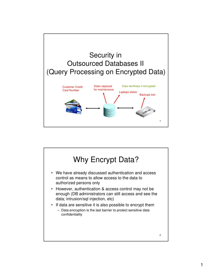
Security in Outsourced Databases II Outsourced Databases II (Query Processing on Encrypted Data)

Customer Credit Card Number Disks replaced for maintenance Laptops stolen Backups lost Data worthless if encrypted

1

p

Why Encrypt Data?

• We have already discussed authentication and access

control as means to allow access to the data to control as means to allow access to the data to authorized persons only

• However, authentication & access control may not be

enough (DB administrators can still access and see the data; intrusion/sql injection, etc)

• If data are sensitive it is also possible to encrypt them

Data encryption is the last barrier to protect sensitive data – Data encryption is the last barrier to protect sensitive data confidentiality

2

2

Why Encypt Data? - External requirements

• Health Insurance Portability & Accountability

Act (HIPPA):

– Requires data safeguards that protect against “intentional

• r unintentional use or disclosure of protected health

information” – It mandates “to ensure the confidentiality, integrity and availability of all electronic protected health information the covered entity creates, receives, maintains, or transmits” – It mandates “to implement a mechanism to encrypt and decrypt electronic protected health information”

3

Why Encypt Data? - Business Compliance

• Payment Card Industry (PCI) Data

S it St d d Security Standard

– Stored cardholder data must be rendered unreadable, and it includes cryptographic methods in the recommended controls – Adopted by American Express, Visa, MasterCard and several other payment card companies p y p

4

3

Three options for database encryption

5 SQL Server TDE (Transparent Data Encryption) Oracle 10g/11g TDE

Can we offer better performance?

 We DO NOT fully trust the service provider with sensitive

information

 Encrypt client’s data and store at server  Encrypt client s data and store at server  Client:  runs queries over encrypted remote data  verifies integrity/authenticity of results (covered in the last lecture)

 Most of the processing work to be done by the server  Consider passive adversary

A li i i di id l h h t d t b t l t i t l

6

 A malicious individual who has access to data but only tries to learn

sensitive information about the data without actively modifying it or disrupting any kind of services

4

Service Provider Architecture

Server Site

Result Filt Encrypted Results

Client Site

(5) (6a) Encrypted Query Translator Temporary Results Filter Server Side Query Service Provider Client Side Query

?

Client Side Query Server Side Query (2) (3) (4) (7) (6b)

7

Database Metadata Original Query Actual Results User

? ?

Original Query (1)

• H. Hacigumus, B. R. Iyer, C. Li, S. Mehrotra: Executing SQL over encrypted data in the database-service-provider model.

2002 International Conference on Management of Data (SIGMOD'2002), 216-227

Query Processing 101…

• At its core, query processing consists of:

– Logical comparisons (> , <, = , <=, >=) – Pattern based queries (e.g., *Arnold*egger*) – Simple arithmetic (+, *, /, ^, log)

• Higher level operators implemented using the

above

– Joins – Selections – Unions S diff

8

– Set difference – …

• To support any of the above over encrypted data,

need to have mechanisms to support basic

• perations over encrypted data

5

Searching over Encrypted Data

• Want to be able to perform operations over encrypted

data (for efficiency)

SELECT AVG(E salary) SELECT AVG(E.salary) FROM EMP WHERE age > 55

• Fundamental observations

– Basic operations do not need to be fully implemented over encrypted data – To test (AGE > 55), it might suffice to devise a strategy that

9

To test (AGE 55), it might suffice to devise a strategy that allows the test to succeed in most cases (might not work in all cases) – If test does not result in a clear positive or negative over encrypted representation, resolve later at client-side, after decryption.

Relational Encryption

NAME SALARY PIN

etuple N ID S ID P ID

Server Site

NAME SALARY PIN

John

50000

2 Mary 110000 2 James 95000 3 Lisa 105000 4 etuple N_ID S_ID P_ID fErf!$Q!!vddf>></| 50 1 10 F%%3w&%gfErf!$ 65 2 10 &%gfsdf$%343v<l 50 2 20 %%33w&%gfs##! 65 2 20

10



Store an encrypted string – etuple – for each tuple in the original table

 This is called “row level encryption”  Any kind of encryption technique (e.g., AES, DES) can be used 

Create an index for each (or selected) attribute(s) in the original table

6

Building the Index

• Partition function divides domain values into partitions (buckets)

Partition (R.A) = { [0,200], (200,400], (400,600], (600,800], (800,1000] } – partition function has impact on performance as well as privacy – very much domain/attribute dependent – equi-width vs. equi-depth partitioning

200 400 600 800 1000 2 7 5 1 4 Partition (Bucket) ids

• Identification function assigns a partition id to each partition of attribute

A

11 200 400 600 800 1000 Domain Values

• e.g. identR.A( (200,400] ) = 7
• Any function can be use as identification function, e.g., hash functions
• Client keeps partition and identification functions secret (as metadata)
• Mapping function maps a value v in the domain of

attribute A to partition id

Building the Index

200 400 600 800 1000 2 7 5 1 4 Domain Values Partition (Bucket) ids 12

– e.g., MapR.A( 250 ) = 7 MapR.A( 620 ) = 1

7

Storing Encrypted Data

R = < A, B, C >  RS = < etuple, A_id, B_id, C_id > etuple = encrypt ( A | B | C ) A_id = MapR.A( A ), B_id = MapR.B( B ), C_id = MapR.C( C )

NAME SALARY PIN

John 50000 2 Etuple N_ID S_ID P_ID fErf!$Q!!vddf>></| 50 1 10

Table: EMPLOYEE Table: EMPLOYEES

13

Mary 110000 2 James 95000 3 Lisa 105000 4 F%%3w&%gfErf!$ 65 2 10 &%gfsdf$%343v<l 50 2 20 %%33w&%gfs##! 65 2 20

Referring back to our example

SELECT AVG(E.salary) FROM EMP WHERE age > 55 WHERE age 55

• Suppose the partitions on age are as follows: P1 - [20,30); P2 -

[30,40); P3 - [40,50); P4 - [50,60); P5 - [60,100)

• To test (AGE > 55), it suffices to retrieve all data that falls into

partitions that contain at least one employee with age > 55

– P4 and P5 – These partitions (e g P4) may contain records with age  55; they can be

14

These partitions (e.g., P4) may contain records with age  55; they can be examined at the client-side after records are decrypted.

• Records belonging to partitions that contain only employees with

age  55 (e.g., P1, P2 and P3) will not need to be returned.

8

Mapping Conditions

Q: SELECT name, pname FROM employee, project WHERE employee.pin=project.pin AND salary>100k

• Server stores attribute indices determined by mapping functions
• Client stores metadata and uses it to translate the query

Conditions:

• Condition  Attribute op Value
• Condition  Attribute op Attribute
• Condition  (Condition  Condition) | (Condition  Condition)

15

Co d t o  (Co d t o Co d t o ) | (Co d t o Co d t o ) | (not Condition) Where op = { = , >, , <,  }

Mapping Conditions (2)

Example: Equality

• Attribute = Value

– Mapcond( A = v )  AS = MapA( v ) – Mapcond( A = 250 )  AS = 7

Partition Ids 16 200 400 600 800 1000 2 7 5 1 4 210 355 250 390

At client site

9

Mapping Conditions (3)

Example: Inequality (<, >, etc.)

• Attribute < Value

– Mapcond( A < v )  AS  { identA( pj) | pj.low  v) } – Mapcond( A < 250 )  AS  {2,7}

Partition Ids

17

200 400 600 800 1000 2 7 5 1 4 Domain Values

210 355 234 390

At client site

Mapping Conditions (4)

• Attribute1 = Attribute2 (useful for JOIN-type queries)

Map ( A = B )   (AS = ident ( )  BS = ident ( )) – Mapcond( A = B )  N (AS = identA( pk )  BS = identB( pl )) where N is pk  partition (A), pl  partition (B), pk  pl  

Partitions A_id [0,100] 2 (100,200] 4 Partitions B_id [0,200] 9 (200,400] 8

18

(200,300] 3 C : A = B  C’ : (A_id = 2  B_id = 9)  (A_id = 4  B_id = 9)  (A_id = 3  B_id = 8)

10

Relational Operators over Encrypted Relations

• Partition the computation of the operators across client

and server C t ( ibl ) t f t th

• Compute (possibly) superset of answers at the server
• Filter the answers at the client
• Objective : minimize the work at the client and process the

answers as soon as they arrive requiring minimal storage at the client Operators:

19

p

– Selection – Join – Grouping and Aggregation – Others: Sort, duplicate elimination, set difference, union, projection

Selection Operator

c( R ) = c( D (

S

Mapcond(c)( R

S ) )

D = Decrypt

A=250

TABLE

Example:

A=250

D

A_id = 7

Client Query

20 200 400 600 800 1000 2 7 5 1 4

E_TABLE Server Query

11

Selection Operator

c( R ) = c( D (

S

Mapcond(c)( R

S ) )

N ll A D = Decrypt

E# A# 2 120

A=250

TABLE

Example:

A=250

D

A_id = 7

Client Query

etuple A# 2%$&* 2 D(6*&^%) = 240 D(8***^%) = 300

Null Answer

21 6 240 8 300 12 500 200 400 600 800 1000 2 7 5 1 4

E_TABLE Server Query

6*&^% 7 8***^% 7 12#@! 5

Join Operator

R c T = c( D ( R

S S

Mapcond(c) T

S )

Client Query

C

EMP PROJ

Example:

C’

E_EMP E_PROJ

A=B

D Server Query

22 C : A = B  C’ :(A_id = 2  B_id = 9)

 (A_id = 4  B_id = 9)  (A_id = 3  B_id = 8) Partitions A_id [0,100] 2 (100,200] 4 (200,300] 3 Partitions B_id [0,200] 9 (200,400] 8

Q y

12

Join Operator

C : A = B  C’ :(A_id = 2  B_id = 9)

 (A_id = 4  B_id = 9)  (A_id = 3  B_id = 8) R c T = c( D ( R

S S

Mapcond(c) T

S )

Client Query

C

EMP PROJ

Example:

C’

E_EMP E_PROJ

A=B

D Server Query

23 P1# Partition A_id 10 (0,100] 2 30 (0,100] 2 120 (100,200] 4 250 (200,300] 3 P2# Partition B_id 70 (0,200] 9 120 [0,200] 9 220 (200,400] 8

P1# P2# 10 70 10 120 30 70 30 120 120 70 120 120 250 220

Condition: P1# = P2#

Join Operator

C : A = B  C’ :(A_id = 2  B_id = 9)

 (A_id = 4  B_id = 9)  (A_id = 3  B_id = 8) R c T = c( D ( R

S S

Mapcond(c) T

S )

Client Query

C

EMP PROJ

Example:

C’

E_EMP E_PROJ

A=B

D Server Query

24 P1# Partition A_id 10 (0,100] 2 30 (0,100] 2 120 (100,200] 4 250 (200,300] 3 P2# Partition B_id 70 (0,200] 9 120 [0,200] 9 220 (200,400] 8

P1# P2# 10 70 10 120 30 70 30 120 120 70

120 120

250 220

Condition: P1# = P2#

13

Grouping & Aggregation Operator

L(R) = L( D ( L’ ( R

S) ) )

where L = { grouping attributes}  { aggregate operations}

EMP

Example:

D Client Query

did, COUNT(eid) S

did S

did, COUNT(eid)

25

EMP E_EMP Server Query

a) Partial sorting done at server b) No gain in terms of communication, but client side saves up on sorting

Query Decomposition

Q: SELECT name, pname FROM emp, proj WHERE emp.pid=proj.pid AND salary > 100k

Client Query



l 100k

name,pname

D

e.pid = p.pid

name,pname

e.pid = p.pid 26

Server Query Encrypted (EMP) Encrypted (PROJ)

salary >100k

D EMP PROJ

salary >100k

14

Query Decomposition (2)

Client Query

name,pname

Client Query

salary >100k

D

e.pid = p.pid

name,pname

Client Query

salary >100k

D D

e.pid = p.pid 27

E_EMP E_PROJ D Server Query E_EMP E_PROJ

s_id = 1 v s_id = 2

Server Query

Query Decomposition (3)

name,pname

Client Query

name,pname

Client Query

e.pid = p.pid

salary >100k

D D

MapCond(e.p id =

salary >100k  e.pid = p.pid

D

28

E_EMP E_PROJ

s_id = 1 v s_id = 2

Server Query

p ( p_ p.p_id)

E_EMP E_PROJ

s_id = 1 v s_id = 2

Server Query

15

Query Decomposition (4)

Q: SELECT name, pname

FROM emp, proj WHERE emp.pid=proj.pid

name,pname

Client Query

p p p j p AND salary > 100k

QS: SELECT e_emp.etuple, e_proj.etuple

FROM e_emp, e_proj WHERE e.p_id=p.p_id AND (s_id = 1 OR s_id = 2)

MapCond(e.p_id = p p id)

salary >100k  e.pid = p.pid

D

29

QC: SELECT

name, pname FROM temp WHERE emp.pid=proj.pid AND salary > 100k

p.p_id)

E_EMP E_PROJ

s_id = 1 v s_id = 2

Server Query

Temp = Decrypted intermediate result

Query Precision vs. Privacy

Observation:

Allocating a large number of buckets to crypto-indices increases query precision but reduces

• privacy. On the other hand, a small number of buckets

increases privacy but adversely affects performance.

The goal of the client is thus twofold:

Server Efficiency: maximize the server-side ac- curacy of range query evaluation. Higher efficiency results in lower server-client communication overhead

30

and lower post-processing costs for the client. Maximum Privacy: minimize the information re- vealed to the server through the crypto-indices. In

• ther words, maximize data privacy.

16

Fine Encryption Granularity

Table: EMPLOYEE Table: EMPLOYEES NAME SAL COM

John 50000 5000 Mary 110000 11000 James 95000 9500 Lisa 105000 10500

Table: EMPLOYEE Table: EMPLOYEE E_NAME E_SAL E_COM

45ewt*(& 3t45f33 *&%*kk (*#hKJ(0 Ek%98* !DE#$F ()&%^JK H^F(j^7 %^g%6 324(&^hj (86&&h$ 887^%$

31

• H. Hacigumus, B. R. Iyer, C. Li, S. Mehrotra: Efficient Execution of Aggregation Queries over Encrypted Relational Databases.

DASFAA04, 125-136

Can we do better with aggregation?

• Use homomorphic encryption functions

– E (encryption function), D (decryption function) –  = {1, 2, …, n} (functions on plaintext), –  = {1, 2, … n} (functions on encrypted data) – (E, D, , ) is a privacy homomorphism if

• D(i(E(a1),E(a2),…, E(am))) = i(a1, a2, …, am)

32

(i( (

1), ( 2),

, (

m))) i( 1, 2,

,

m)

17

Aggregation over encrypted data

• One such scheme

Key k (p q) p & q are prime numbers chosen by – Key k = (p,q), p & q are prime numbers chosen by client used for encryption/decryption (hidden from server) – N = p.q, revealed to server – Ek(a) = (a mod p, a mod q), a  N – Dk(d1, d2) = d1qq-1 + d2pp-1 (mod N)

33

• qq-1 = 1 (mod p), pp-1 = 1 (mod q)

–  = {n, n, n} –  = {, , }

Aggregation over encrypted data

• Example

– p = 5, q = 7, so N = pq = 35, k = (5, 7) – Suppose we want to add a1=5 and a2=6 – Ek(5) = (0,5), Ek(6) = (1,6) (stored in server) – At server

• Compute Ek(5) + Ek(6) = (1,11)

34

– At client

• Decrypts (1,11) = (1.7.3 + 11.5.3) (mod 35) = 11 = 5 + 6!

18

In relational DBMS

• For each attribute A that will be used in aggregation, create two

fields to encode E(a), a  domain(A), e.g., for salary, we create Sp = salary mod p and Sq = salary mod q Now SUM(salary + commission) can be processed at the server as

NAME SAL COM

Etuple Sp Sq Cp Cq

Table: EMPLOYEE Table: EMPLOYEES

• Now SUM(salary + commission) can be processed at the server as

– SELECT SUM(Sp+Cp) as s1, SUM(Sq+Cq) as s2 FROM EMPS

• Client decrypts result as

– S1*q*q-1 + s2*p*p-1 (mod p*q)

35

NAME SAL COM

John 50000 5000 Mary 110000 11000 James 95000 9500 Lisa 105000 10500 Etuple Sp Sq Cp Cq fErf!$Q!!vddf 34 24 63 23 F%%3w&%g 56 26 34 22 &%gfsdf$%3 25 55 47 44 %%33w&%gf 86 33 42 92

Complete example

eid name salary city did 23 Tom 70K Maple 10 860 John 60K Maple 55 Salary Paritions ID 0-25K 59

etuple S_id City_id Did_id E_city E_did Sal_p Sal_q

fErf!$Q! 81 18 2 **^(( @R@* 7 27 860 Jo 60 ap e 55 320 Jim 23K River 35 875 Tim 45K Maple 58 870 Mary 40K Maple 10 200 Susan 45K Ruver 10 5 59 25K-50K 49 50K-75K 81 75K-100K 7

SalaryPH

36

$Q 8 8 (( @ @ F%%3g 81 18 3 **^(( (&%^4 18 17 &%gfsd 59 22 4 Il23^ $(7%$ 2 23 ^#$#%^ 49 18 3 **^(( #%&*9 3 2 %%33w 49 18 2 **^(( @R@* 8 7 fErf!Q!! 49 22 2 Il23^ @R@* 13 12

19

Select SUM(Salary) FROM emp, mgr WHERE city=Maple AND salary< 65K and emp.did = mgr.did

• For city=Maple, we use E_city
• For salary < 65K, we use

S id 49 OR S id 59 ( f l d ) – S_id = 49 OR S_id = 59 (no false drop) – S_id = 81 (false drop exists)

• For emp.did = mgr.did, we use E_did
• So, we can have TWO subqueries at the server (why?)

– SELECT SUMPH(SalaryPH) FROM empS, mgrS WHERE E_city=E(Maple) AND (S_id=49 OR S_id=59) AND empS.E_did=mgrS.E_did SELECT empS etuple FROM empS mgrS WHERE E city=E(Maple) AND

37

– SELECT empS.etuple FROM empS, mgrS WHERE E_city=E(Maple) AND S_id=81 AND empS.E_did=mgrS.E_did

• Client?

Summary

• Store encrypted data at server
• Process as much at server as possible, and

t t li t postprocess at client

• Storage cost is higher (hash values can be as

large as the original values)

• Leak some information

– number of distinct values, which records have the same values in certain attribute, which records are

38

, join-able, – violate access control

• Effectiveness depends on the partitioning/index

granularity