Which models can be fit with linear regression? Simple linear - PowerPoint PPT Presentation

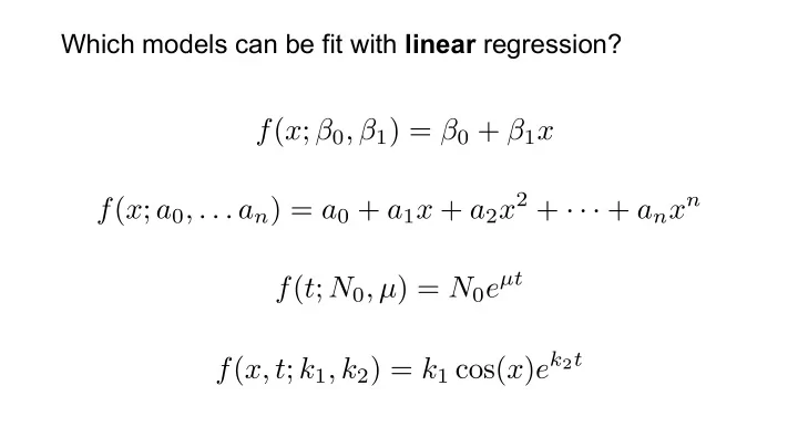
Which models can be fit with linear regression?

Simple linear regression in Matlab X = rand(3,3) b = pinv(X) * y X = b = 0.0467 0.5188 0.5317 14.3966 0.6587 0.3323 0.5070 50.9428 0.7573 0.0428 0.2532 -50.8102 y = rand(3,1) b = X \ y y = b = 0.0820 14.3966 0.6530 50.9428 0.2190 -50.8102

Simple linear regression

Simple linear regression b = x \ y b = 11.3784 scatter ( x,y ); hold on ; plot ( x , b .* x ); title (' y = \beta_1 x' , 'FontSize' ,18); hold off ;

Simple linear regression b = [ ones ( size ( x )) x ] \ y b = -42.1779 15.5615 scatter ( x,y ); hold on ; plot ( x , b (1) + b (2)* x ); title (' y = \beta_0 + \beta_1 x '); hold off ;

Simple linear regression b = [ ones ( size ( x )) x x.^2] \ y b = -2.6376 2.1967 0.8353 scatter ( x,y ); hold on ; plot ( x , b (1) + b (2)* x + b(3)*x.^2); title (' y = \beta_0 + \beta_1 x + \beta_2 x^2 '); hold off ;

Easier modeling with fitlm 1. Create a Matlab table Column names are taken from the names of the variables in the call to tbl = table(x,y) table. To use other names set tbl = 100×2 table x y tbl.Properties.VariableNames = {'name1', 'name2'} ______ ________ tbl = 100×2 table name1 name2 1 0.07747 ______ ________ 1.1414 10.604 1 0.07747 1.2828 0.24382 1.1414 10.604 1.4242 0.066588 1.2828 0.24382 1.5657 2.3857 1.4242 0.066588 1.5657 2.3857 1.7071 9.643 1.7071 9.643 1.8485 1.2993 1.9899 6.4243 2.1313 6.2049

Easier modeling with fitlm fitlm(tbl, 'y~x') model = Linear regression model: y ~ 1 + x Estimated Coefficients: Estimate SE tStat pValue ________ _______ _______ __________ (Intercept) -42.178 4.4325 -9.5157 1.3623e-15 x 15.561 0.49352 31.531 4.1479e-53 Number of observations: 100, Error degrees of freedom: 98 Root Mean Squared Error: 20.1 R-squared: 0.91, Adjusted R-Squared 0.909 F-statistic vs. constant model: 994, p-value = 4.15e-53

Easier modeling with fitlm plot(model)

Easier modeling with fitlm model2 = fitlm(tbl, 'y~x^2') model2 = Linear regression model: y ~ 1 + x + x^2 Estimated Coefficients: Estimate SE tStat pValue ________ _______ ________ _________ (Intercept) -2.6376 6.1135 -0.43145 0.6671 x 2.1967 1.7424 1.2608 0.21042 x^2 0.8353 0.10617 7.8676 5.123e-12 Number of observations: 100, Error degrees of freedom: 97 Root Mean Squared Error: 15.8 R-squared: 0.945, Adjusted R-Squared 0.944 F-statistic vs. constant model: 837, p-value = 6.61e-62

Easier modeling with fitlm plot(model2)

Exploratory Data Analysis with Linear Regression load hospital hospital(1:10,:) ans = LastName Sex Age Weight Smoker BloodPressure Trials YPL-320 'SMITH' Male 38 176 true 124 93 [ 18] GLI-532 'JOHNSON' Male 43 163 false 109 77 [1×3 double] PNI-258 'WILLIAMS' Female 38 131 false 125 83 [1×0 double] MIJ-579 'JONES' Female 40 133 false 117 75 [1×2 double] XLK-030 'BROWN' Female 49 119 false 122 80 [1×2 double] TFP-518 'DAVIS' Female 46 142 false 121 70 [ 19] LPD-746 'MILLER' Female 33 142 true 130 88 [ 13] ATA-945 'WILSON' Male 40 180 false 115 82 [1×0 double] VNL-702 'MOORE' Male 28 183 false 115 78 [ 2] LQW-768 'TAYLOR' Female 31 132 false 118 86 [ 11] hospital.meanBP = mean(hospital.BloodPressure, 2); hospital(1:10,:) ans = LastName Sex Age Weight Smoker BloodPressure Trials meanBP YPL-320 'SMITH' Male 38 176 true 124 93 [ 18] 108.5 GLI-532 'JOHNSON' Male 43 163 false 109 77 [1×3 double] 93 PNI-258 'WILLIAMS' Female 38 131 false 125 83 [1×0 double] 104 MIJ-579 'JONES' Female 40 133 false 117 75 [1×2 double] 96 XLK-030 'BROWN' Female 49 119 false 122 80 [1×2 double] 101 TFP-518 'DAVIS' Female 46 142 false 121 70 [ 19] 95.5 LPD-746 'MILLER' Female 33 142 true 130 88 [ 13] 109 ATA-945 'WILSON' Male 40 180 false 115 82 [1×0 double] 98.5 VNL-702 'MOORE' Male 28 183 false 115 78 [ 2] 96.5 LQW-768 'TAYLOR' Female 31 132 false 118 86 [ 11] 102

Exploratory Data Analysis with Linear Regression fitlm(hospital, 'meanBP ~ Sex + Age + Weight + Smoker') ans = Linear regression model: meanBP ~ 1 + Sex + Age + Weight + Smoker Estimated Coefficients: Estimate SE tStat pValue __________ ________ _________ __________ (Intercept) 97.09 5.4093 17.949 2.7832e-32 Sex_Male 0.51095 2.0897 0.24451 0.80737 Age 0.058337 0.047726 1.2224 0.2246 Weight -0.0008026 0.039503 -0.020317 0.98383 Smoker_1 10.088 0.73786 13.672 3.6239e-24 Number of observations: 100, Error degrees of freedom: 95 Root Mean Squared Error: 3.41 R-squared: 0.683, Adjusted R-Squared 0.67 F-statistic vs. constant model: 51.2, p-value = 6.55e-23