What have we learnt about inflation from WMAP ? Courtesey: NASA/WMAP - - PowerPoint PPT Presentation

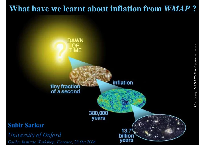
What have we learnt about inflation from WMAP ?

Courtesey: NASA/WMAP Science Team

Subir Sarkar University of Oxford

Galileo Institute Workshop, Florence, 23 Oct 2006

‘Internal Linear Combination’ map (circa March 2006)

Coherent oscillations in photon-baryon plasma, excited by primordial density perturbations on super-horizon scales … (Hubble radius at trec) Cl’s mildly correlated since (due to Galactic foreground)

• nly ~85% of sky can be used

WMAP 3-yr WMAP 1-yr

θ ~1800/l

S/N > 1 for

ℓ > 850

WMAP does provide evidence for inflation …

The characteristic features of scalar density perturbations generated during a (quasi-) de Sitter phase of expansion: (a) Coherence of the Fourier modes clean ‘acoustic peak’ structure on angular scales (< 10) which were sub-Hubble radius at last scattering (z ~ 103) (b) Dipole out-of-phase with the monopole negative cross-correlation between temperature and (electric) polarization on (super- Hubble radius) scales ~1-50

cosmic variance limited for ℓ < 400

see Dodelson (2003)

Observations of large-scale structure are consistent with the ΛCDM model if the primordial fluctuations are adiabatic and ~scale-invariant (as is apparently “expected in the simplest models of inflation”)

• Tegmark. (2004)

CMB (+ LSS) data indicates that inflation generated adiabatic, ~scale-invariant scalar density perturbations

But no tensor perturbations have yet been detected (through the expected B-mode polarization at low l) … can only set crude limit: r T/S < 0.55

⇒ Bound on inflationary energy scale: V1/4 < 2 x 1016 GeV … thus no specific clue to the physics driving inflation (GUT-scale? Hidden-sector scale? Electroweak scale?)

Can at best attempt to rule out ‘toy models’ (e.g. V = λφ4) where inflation occurs at φ > ΜP hence a large tensor signal is predicted … Is there any signature in the data of the physics responsible for inflation? … can discuss this sensibly only in the context of an effective field theory i.e. with φ << ΜP …

But neither model has a physical basis (φ >MP!) and both are fine-tuned: λ ~ 10-12 or m/MP ~ 10-6 to generate the density perturbation δH ~ 10-5 ...

WMAP-3 prefers V = m2φ 2 over V = λφ4

What we measure is the density perturbation, not the inflaton potential

⇒ ⇒ ⇒ ⇒

If the linear term in the expansion of V(φ) dominates, then So the energy scale required to generate δH ~ 10-5 is indeed ~ MGUT:

• n the scale k which exits the horizon when φ∗ = φ∗

H:

… so expand this around the field value φ∗

I when the perturbation just

entering our present Hubble radius (H0

• 1 ~ 3000 h-1 Mpc) was generated

Then:

Question: What sort of models exhibit “linear inflation”? Answer: All “chaotic” (large-field) models with because then: so V = m2φ 2,λφ 4 are both equivalent to: V V(0) + αφ But if φ transforms under a symmetry then no linear term “new inflation” with

⇒

So the energy scale of inflation gets smaller as φΗ 0:

German, Ross & Sarkar (2001)

...can generate adequate inflation with correct δ δ δ δH at any energy scale Effective field theory: mass term + non-renormalizable operators

Energy Scale (GeV) # e-folds

requires b < 1/20 (cf. ‘natural’ value: ~1 ⇒ “η problem”) General ‘new’ inflaton potential:

Inflation at SUGRA ‘hidden-sector’ scale Inflation at QCD scale The required NR operator can be realised in a physical theory

Best-fit: mh2 = 0.13 ± 0.01, bh2 = 0.022 ± 0.001, h = 0.73 ± 0.05, n = 0.95 ± 0.02

The 3-yr WMAP data is said to confirm the ‘power-law ΛCDM model’

But the χ χ χ χ2/dof = 1049/982 ⇒ ⇒ ⇒ ⇒ probability of only ~7% that this model is correct!

The excess 2 comes mostly from the outliers in the TT spectrum

“glitches”

?

WMAP-1: Only 3 out of 16000 simulations would have a lower value of C181 than that observed (Lewis 2004)

Similar outliers have been seen by Archeops (although less significant)

Is the primordial density perturbation really scale-free? glitches?

“In the absence of an established theoretical framework in which to interpret these glitches … they will likely remain curiosities” Spergel et al (2006) “In the absence of an established theoretical framework in which to interpret dark energy … the apparent acceleration of the universe will likely remain a curiosity” Then why not also say:

The formation of large-scale structure is akin to a scattering experiment The Beam: inflationary density perturbations

No ‘standard model’ – usually assumed to be adiabatic and ~scale-invariant

The Target: dark matter (+ baryonic matter)

Identity unknown - usually taken to be cold (sub-dominant ‘hot’ component?)

The Signal: CMB anisotropy, galaxy clustering …

measured over scales ranging from ~ 1 – 10000 Mpc (⇒ ~8 e-folds of inflation)

The Detector: the universe

Modelled by a ‘simple’ FRW cosmology with parameters h, CDM , b , , k ...

We cannot simultaneously determine the properties of both the beam and the target with an unknown detector … hence need to adopt suitable ‘priors’ on h, CDM, etc in order to break inevitable parameter degeneracies

Astronomers have traditionally assumed a Harrison-Zeldovich spectrum: P(k) ∝ kn, n = 1 But models of inflation generally predict departures from scale-invariance In single-field slow-roll models: n = 1 + 2V/ V – 3 (V/V)2 Since the potential V(φ) steepens towards the end of inflation, there will be a scale-dependent spectral tilt on cosmologically observable scales: e.g. in model with cubic leading term: V(φ) ≃ Vo − φ3 + … ⇒ n ≃ 1 – 4/N* ~ 0.94 where N* ≈ 60 + ln (k-1/3000h-1 Mpc) is the # of e-folds from the end of inflation In hybrid models, inflation is ended by the ‘waterfall’ field, not due to the steepening of V(φ), so spectrum is generally closer to scale-invariant … In general there would be many other fields present, whose own dynamics may interrupt the inflaton’s slow-roll evolution (rather than terminate it altogether) can generate features in the spectrum (‘steps’, ‘oscillations’, ‘bumps’ …) This agrees with the best-fit value power-law index inferred from the WMAP data

Many attempts made to reconstruct the primordial spectrum (assuming CDM)

Bridle, Lewis, Weller & Efstathiou 2003; Cline, Crotty & Lesgourgues 2003, Mukherjee & Wang 2003; Hannestad 2004; Kogo, Sasaki & Yokoyama 2004; Tocchini-Valentini, Douspis & Silk 2004, …

… Essential to use non-parametric methods (Shafieloo & Souradeep 2004)

Tochhini-Valentini, Hoffman & Silk (2005) IR cutoff at present Hubble radius? Damped oscillations? WMAP-1 “best-fit” P = k0.97

Such spectra arise naturally if the inflaton mass changes suddenly, e.g. due to its coupling (through gravity) to a field which undergoes a fast symmetry-breaking phase transition in the rapidly cooling universe

(Adams, Ross & Sarkar 1997)

This must happen as cosmologically interesting scales ‘exit the horizon’ ... likely if (last phase of) inflation did not last longer than ~50-60 e-folds

Hunt & Sarkar (2005)

Consider inflation in context of effective field theory: N =1 SUGRA

(successful description of gauge coupling unification, EW symmetry breaking, …)

These fields get a large mass ( These fields get a large mass ( These fields get a large mass ( These fields get a large mass (m m m m2

2 2 2 ~

~ ~ ~ ± ± ± ±H H H H2

2 2 2)

) ) ) during during during during inflation, thus perturbing the inflaton inflation, thus perturbing the inflaton inflation, thus perturbing the inflaton inflation, thus perturbing the inflaton

All this happens if the initial conditions are thermal initial conditions are thermal initial conditions are thermal initial conditions are thermal (i.e. ρ starts at origin) and this (last) phase of inflation lasts just long enough inflation lasts just long enough inflation lasts just long enough inflation lasts just long enough to create present Hubble volume to create present Hubble volume to create present Hubble volume to create present Hubble volume may seem fine-tuned but the data does indicate an IR cutoff IR cutoff IR cutoff IR cutoff at the present Hubble radius!

Use WKB method ( Use WKB method ( Use WKB method ( Use WKB method (Martin & Schwarz 2003 Martin & Schwarz 2003 Martin & Schwarz 2003 Martin & Schwarz 2003) to obtain ) to obtain ) to obtain ) to obtain P P P PR

R R R when slow

when slow when slow when slow-

• roll is violated

roll is violated roll is violated roll is violated … … … …

Fits are all acceptable but fit parameters change little except for large-scale amplitude

Hunt & Sarkar (2006)

Measurable in galaxy surveys?

WMAP does not require the primordial density perturbation to be scale-free!

Parameter degeneracies - ΛCDM universe (‘step’ spectrum)

Hunt & Sarkar (to appear)

MCMC likelihood distributions for ΛCDM (‘step’ spectrum) … not too different from ‘power law ΛCDM’

Hunt & Sarkar (to appear)

But if there are many flat direction fields, then two phase transitions may

• ccur in quick succession, creating a

‘bump’ in the primordial spectrum on cosmologically relevant scales

The WMAP data can then be fitted just as well with no dark energy (m = 1, = 1, = 1, = 1, Λ

Λ Λ Λ = 0,

= 0, = 0, = 0, h = 0.46)

h = 0.46 is inconsistent with Hubble Key Project value (h = 0.72 ± 0.08)

but is in fact indicated by direct (and much deeper) determinations e.g. gravitational lens time delays (h = 0.48 ± 0.03) Best fit CDM model Low h EdeS

Blanchard et al (2003)

Suggests expansion rate may be 30% higher locally than globally!

HKP depth

Are we located in a ~500 Mpc void which is expanding faster than the average rate (inhomogeneous Lemaitré-Tolman-Bondi model)? Can the ‘Rees-Sciama effect’ due to our local inhomogeneity then explain the mysterious alignment of the quadrupole and octupole?

(e.g. Inoue & Silk 2006)

The Lemaitré-Tolman-Bondi model may even explain the SNIa Hubble diagram without acceleration!

Biswas, Mansouri & Notari (2006)

CDM ‘Gold dataset’ EdeS LTB

The small-scale power would be excessive unless damped by free-streaming ... Adding 3 ν ν ν νs of mass 0.8 eV (⇒ ⇒ ⇒ ⇒Ω Ω Ω Ων

ν ν ν≈

≈ ≈ ≈ 0.14) gives good match to large-scale structure Fit gives Ωbh2 ≈ 0.021 → BBN √ √ √ √ ⇒ baryon fraction in clusters predicted to be ~11% √ √ √ √

SDSS

( ( ( (note that Σ Σ Σ Σ mν

ν ν ν ≈

≈ ≈ ≈ 2.4 eV – well above ‘WMAP bound’!)

Parameter degeneracies - CHDM universe (‘bump’ spectrum)

Hunt & Sarkar (to appear)

MCMC likelihoods - CHDM universe (‘bump’ spectrum)

Hunt & Sarkar (to appear) This is ~50% higher than the ‘WMAP value’ used widely for CDM abundance To fit the large- scale structure data requires ~eV mass neutrinos Consistent age for the universe Consistent with data on clusters and weak lensing

New Test: Baryon Acoustic Peak in the Large-Scale Correlation Function of SDSS Luminous Red Galaxies ~1% excess of galaxies at separation of ~150 Mpc

In EdeS model with no dark energy, the baryon bump is at the ~same physical scale, but at a different location in observed (redshift) space

We can match the angular size of the 1st acoustic peak at z ~ 1100 by taking h ~ 0.5, but we cannot then also match the angular size of the baryonic feature at z ~ 0.35

But for inhomogeneous LTB model (h ~ 0.7 for z < 0.08, then h 0.5) angular diameter distance @ z = 0.35 is similar to Λ Λ Λ ΛCDM!

Biswas, Mansouri, Notari (2006)

WMAP is supposed to have confirmed the need for a dominant component of dark energy from precision observations of the CMB However we cannot simultaneously determine both the primordial spectrum and the cosmological parameters from CMB (and LSS) data We do not know the physics behind inflation hence are not justified in assuming that the generated scalar density perturbation is scale-free (and then conclude that the data confirm the power-law ΛCDM model) The data provides intriguing hints for features in the primordial spectrum … this has crucial implications for parameter extraction e.g. a ‘bump’ in the spectrum allows the data to be well-fitted without any dark energy! Given the unacceptable degree of fine-tuning required to accommodate dark energy, we should explore if the SNIa Hubble diagram, BAO etc can be equally well accounted for in the inhomogeneous LTB model The FRW model may be too simple a description of the real universe!

Conclusions

100 1000

R/(h−1 Mpc)

0.01 0.02 0.03 0.04 0.05 0.06 0.07

Variance of H

LCDM (HZ) LCDM (BSI ’step’) CHDM (BSI ’bump’)

100 1000

R/(h−1 Mpc)

0.05 0.1 0.15 0.2 0.25

Variance of rho

LCDM (HZ) LCDM (BSI ’step’) CHDM (BSI ’bump’)