
SLIDE 1
WMAP 3 years of observations: Methods and cosmological insights
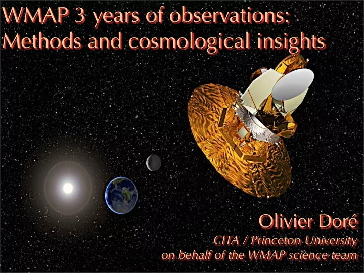
Olivier Doré
CITA / Princeton University
- n behalf of the WMAP science team
WMAP 3 years of observations: Methods and cosmological insights - - PowerPoint PPT Presentation
WMAP 3 years of observations: Methods and cosmological insights Olivier Dor CITA / Princeton University on behalf of the WMAP science team WMAP Science Team NASA - GSFC PRINCETON GODDARD C. Barnes C.Bennett (JHU) R. Bean (Cornell) G.
Olivier Doré
CITA / Princeton University
NASA - GSFC GODDARD
C.Bennett (JHU)
PRINCETON
David Wilkinson 1935-2002
What has WMAP-1 done for us ?
Color codes temperature (intensity), here ±100μK Temperature traces gravitational potential at the time of recombination, when the Universe was 372 000 ±14000 years old The statistical analysis of this map entails detailed cosmological information WMAP-1 has improved over COBE by a factor of 45 in sensitivity and 33 in angular resolution Doing so, the mission met all its requirements after the first year... ”Mission Accomplished!”... but...
What has WMAP-3 done for us?
... the insights expected on Inflation theory (~10-18s after BB) and the Universe reionization (364 +124/-74 Myr) from large scale CMB polarization measurements were too tempting to not be pursued WMAP-3 has measured the CMB polarization on very large angular scales To do so required us to improve control the systematics at a level 50 times higher than originally proposed!
A CMB Primer Recap on WMAP and analysis improvements over the last 2 years A case for large scale polarized CMB detection
Cosmological implications
Phenomenological success of ΛCDM cosmology WMAP already addresses new set of questions risen by this success (Dark Energy, Inflation, Reionization, Non-Gaussianities...)
I can’t cover it all now. Please ask questions and interrupt me!
CMB comes from t=380 000 years after Big Bang Reionization Today: 13.7 Gyrs after Big Bang
The CMB is a leftover from when the Universe was 380 000 yrs old
The Universe is expanding and cooling
Once it is cool enough for Hydrogen to form, (T~3000K, t~3.8 105 yrs), the photons start to propagate freely (the Thomson mean free path is greater than the horizon scale)
This radiation has the imprint of the small anisotropies that grew by gravitational instability into the large structures we see today
Sachs-Wolfe plateau Silk damping Acoustic regime
Θ~π/l
Θ>Θdec~2o
2o 0.5o 0.2o 90o
Confronting sky maps with theoretical predictions
It is both theoretically sound and observationally supported to consider the CMB temperature fluctuations as a gaussian random field so that alm’s are Gaussian random variables Thus sufficient to consider the power spectrum Physics in the linear regime well described by a 3000K plasma photo-baryon fluid
Sunyaev & Zeldovich 70 Peebles & Yu 70 Bond & Efstathiou 87 Hu & White 97
Sachs-Wolfe plateau Silk damping Acoustic regime
Θ~π/l
Θ>Θdec~2o
2o 0.5o 0.2o 90o
S/N per l <1 Cosmic variance >Noise
Confronting sky maps with theoretical predictions
It is both theoretically sound and observationally supported to consider the CMB temperature fluctuations as a gaussian random field so that alm’s are Gaussian random variables Thus sufficient to consider the power spectrum Physics in the linear regime well described by a 3000K plasma photo-baryon fluid
Sunyaev & Zeldovich 70 Peebles & Yu 70 Bond & Efstathiou 87 Hu & White 97
Linear polarization of the CMB is: Produced by Thomson scattering of a quadrupolar radiation pattern on free electrons ⇒probe recombination and reionization Partially correlated with temperature (velocity pert. correlates with density pert.) Two types of Polarization Scalar perturbation to the metric produce E- mode polarization Tensor perturbations to the metric produce B-mode polarization, i.e. Gravity waves Polarization probes both perturbations themselves and ionization history Numerical calculation show that the polarization fraction is weak, ~1% of only
e- e-
WMAP Launch
June 30, 2001 at 3:47 EDT
Delta II Model 7425-10 Delta Launch Number 286 Star-48 third stage motor Cape Canaveral Air Force Station Pad SLC-17B
Trajectory to L2
The spacecraft
Not to scale: Earth — L2 distance is 1% of Sun — Earth Distance
Earth Sun MAP at L2
1 Day 3 Months
6 Months - full sky coverage
129 sec. (0.464rpm) Spin
22.5° half-angle
1hour precession cone A-side line of site B-side line of site Earth-L2 distance 22.5 deg.
Precession rate: 1rph 22.5o half angle Spin rate: 0.464rpm A line of sight B line of sight Earth SUN Lagrange point L2
L2 orbit Constant survey mode Thermal stability Passive cooling Rapid and complex sky scan Observe 30% of the sky every day Most of pixels are observed with evenly distributed
Differential measurement only Most of the common modes cancel Two radiometers per feed T1+T2 ∝ Intensity T1-T2 ∝ Polarization 10 feeds, 20 DA total 5 microwave frequencies to monitor foregrounds K, Ka, Q, V, W bands 22, 33, 40, 60, 93 GHz Accurate calibration on the cosmological dipole and beam measurements on Jupiter Design optimized for temperature measurements
Foreground Spectra
WMAP Sky Maps: 23 to 94 GHz
23 GHz 33 GHz 61 GHz 94 GHz
Absolute Calibration: 0.5% Bandwidth: ~20% Beam FWHM: 0.85˚ (23 GHz) to 0.21˚(94 GHz) Systematic around 15μK2 for C2
TT vs
the ~1000 μK2 nominal TT and ~100 (EE), and less for higher l
41 GHz
K Band (23 GHz)
Temperature (µK)
+200
Ka Band (33 GHz)
Temperature (µK)
+200
Q Band (41 GHz)
Temperature (µK)
+200
V Band (61 GHz)
Temperature (µK)
+200
W Band (94 GHz)
Temperature (µK)
+200
Systematic Error Cross-Checks
(Q1+Q2)/2 (W12-W34)/2 (W12+W34)/2 (V1-V2)/2 (V1+V2)/2 (Q1-Q2)/2
COBE-WMAP Comparison
COBE DMR 53 GHz WMAP Q/V Combined (to approximate 53 GHz)
Temperature (µK)
+100
Difference: WMAP - DMR Simulated DMR Noise (for comparison)
Foreground Removal for Spectrum Analysis
Temperature (µK)
+70
Q V W
External templates Hα maps from Finkbeiner et al. 03 WHAM Haslam et al. 1981 Finkbeiner, Davis & Schlegel 2001
Differential measurement and interlocked scanning strategy suppresses polarization systematics as for temperature. No new systematics, but the weak nature of the spinorial polarized signal requires extra-care to avoid any coupling to the much stronger T field (100 times). Non-trivial interactions between the slow drift gain, non-uniform weighting across the sky, time series masking, 1/f noise, galactic foregrounds, band-pass mismatch, off-set sensitivity and loss imbalance. The handling of these effect had to be propagated from the map-making till the power-spectrum measurement. To understand them required numerous end-to-end simulations (enough to have good statistics). Most of 2004-5 was spent running those and realizing that the previous short-cuts did not work anymore. A new pipeline was eventually required and has been designed, written and
We rely heavily on null tests in map (various frequency) and Cl space to assess the quality of this processing
Remarks on the analysis over the last 2 years
V-band
+200
+30
W-band
V band W band year 1(pub) year 3 year 3 - year 1
Ka band
K band
Q band V band W band
Color code P=(Q2+U2)1/2 smoothed with a 2o fwhm Direction shown for S/N > 1
p02 p06 p04 p08 p10 Sources Dust
0°
+90°
+180° NEP SEP GC
Outside p06 mask
Foregrounds dominate over all l of interest and all frequencies unlike for temperature
Spiral magnetic field structures seen in external galaxies
Bi-symmetric Spiral model
K1 Polarization Amplitude K1 Polarization Prediction from Haslam
0.1 T(mK)
Polarized foregrounds predictions:
synchrotron radiation
180° 0°
Based on a model in which a gas of cosmic rays electrons interact with a magnetic field following a bisymmetric spiral arm pattern
Polarization directions Polarization amplitude
Foreground cleaned maps
pre-cleaned cleaned Q Stokes W-band V-band Q-band Ka-band 20TABLE 4 COMPARISON OF χ2 BETWEEN PRE-CLEANED AND CLEANED MAPS
Due to correlations between foregrounds, a map based cleaning is more powerful 2 parameters/frequency fit only
W 1.38 1.58 6144
Ka 2.142 1.096 4534 4743 Q 1.289 1.018 4534 1229 V 1.048 1.016 4534 145 W 1.061 1.050 4534 50
R a w C l e a n
1 10 100 1000 Multipole moment (l) 0.01 0.10 1.00 10.00 100.00 { l(l+1) Cl / 2 } 1/2 [µK]
Simple ΛCDM model fits
Multipole moment (l) 10 100 500 1000 Angular Scale 2 1 –1 1000 2000 3000 4000 5000 6000 90° 2° 0.5° 0.2° TT TE TESimple flat ΛCDM model with 6 parameters (Ωcdm,Ωb,ns,As,h,τ) still an excellent fit Despite smaller error bars, the χ2eff for TT improves from 1.09 (893 dof) to 1.068 (982 dof) and from 1.066 (1342 dof) to 1.041 for TT+TE (1410 dof) For T, Q, U maps, we have χ2eff=0.981 for 1838 pixels Previously discrepant points get closer
First Year WMAPext Three Year ML ML ML 2.30 2.21 2.22 0.145 0.138 0.128 68 71 73 0.10 0.10 0.092 0.97 0.96 0.958 0.32 0.27 0.24 0.88 0.82 0.77
Driven by EE
0.1 0.2 0.3 0.4 0.5 0.90 0.95 1.00 1.05 1.10 1.15 1.20 1.25
r First Year WMAPext Three Year Mean Mean Mean 2.38+0.13
−0.122.32+0.12
−0.112.23 ± 0.08 0.144+0.016
−0.0160.134+0.006
−0.0060.126 ± 0.009 72+5
−573+3
−374+3
−30.17+0.08
−0.070.15+0.07
−0.070.093 ± 0.029 0.99+0.04
−0.040.98+0.03
−0.030.961 ± 0.017 0.29+0.07
−0.070.25+0.03
−0.030.234 ± 0.035 0.92+0.1
−0.10.84+0.06
−0.060.76 ± 0.05
Parameter 100Ωbh2 Ωmh2 H0 τ ns Ωm σ8
First Year WMAPext Three Year ML ML ML 2.30 2.21 2.22 0.145 0.138 0.128 68 71 73 0.10 0.10 0.092 0.97 0.96 0.958 0.32 0.27 0.24 0.88 0.82 0.77
0.1 0.12 0.14 0.16 0.18 0.2 0.6 0.7 0.8 0.9 1.0 1.1 1.2 1.3 1.4 1.5
Driven by 3d peak
r First Year WMAPext Three Year Mean Mean Mean 2.38+0.13
−0.122.32+0.12
−0.112.23 ± 0.08 0.144+0.016
−0.0160.134+0.006
−0.0060.126 ± 0.009 72+5
−573+3
−374+3
−30.17+0.08
−0.070.15+0.07
−0.070.093 ± 0.029 0.99+0.04
−0.040.98+0.03
−0.030.961 ± 0.017 0.29+0.07
−0.070.25+0.03
−0.030.234 ± 0.035 0.92+0.1
−0.10.84+0.06
−0.060.76 ± 0.05
Parameter 100Ωbh2 Ωmh2 H0 τ ns Ωm σ8
Combination Exact EE Only Exact EE & TE KaQV 0.111±0.022 0.111±0.022 Q 0.100±0.044 0.082±0.043 QV 0.100±0.029 0.092±0.029 QV+VV ··· ··· V 0.089±0.048 0.094±0.043 QVW 0.110±0.021 0.101±0.023 KaQVW 0.107±0.018 0.106±0.019
Formal marginalization give the same results
Cosmological contrasts... and yet concordance
WMAP “predicts” small scale CMB experiments
ACBAR B03 CBI MAXIMA VSA
1000 5000 100 1000 600 400 2000
Cosmological contrasts... and yet concordance
WMAP “predicts” low z mass distribution
(same for 2dF)
The current strong “phenomenological” success means: The primordial inhomogeneities are mostly adiabatic with a nearly scale invariant power spectrum We have a successful GR based theory of linear perturbations to evolve them We have a good description of the main components even if we do not know what they are
We can now ask various sets of questions:
Ask question within the model What else can we learn about the components of the model, eg neutrino? What is Dark Energy? What is Dark Matter? Did the Universe really undergo an Inflationary phase? First stars and how did the Universe get reionized? Explore further the data and look for “anomalies”, ie deviations from this model F u n d a m e n t a l P h y s i c s w e d
’ t k n
y e t P h y s i c s w e d
’ t k n
t
p u t e
Constraints on Neutrino Properties Data Set mν (95% limit for Nν = 3.02) WMAP 2.0 eV(95% CL) WMAP + SDSS 0.91 eV(95% CL) WMAP + 2dFGRS 0.87 eV(95% CL) CMB + LSS +SN 0.68 eV(95% CL)
0.0 1.0 1.5 0.5 2.0 0.5 0.4 0.3 0.6 0.7 0.8 0.9
WMAP WMAP+SDSS
w
0.0 –0.5 –1.0 –1.5 –2.0w
Data Set with perturbations WMAP + SDSS −0.75+0.18
−0.16
WMAP + 2dFGRS −0.914+0.193
−0.099
WMAP + SNGold −0.944+0.076
−0.094
WMAP + SNLS −0.966+0.070
−0.090
CMB+ LSS+ SN −0.926+0.051
−0.075
With DE perturbations
but fixed cs2 (cf Bean & Doré 03)
Constraints on constant DE equation of state w=p/ρ
w + curvature w + neutrino CMB + LSS + SN
–0.08 –0.06 –0.04 –0.02 0.00 0.02 0.04 –1.4 –1.2 –1.0 –0.8
0.0 0.5 1.0 1.5 –1.4 –1.6 –1.2 –1.0 –0.8
Inflation was introduced to solve the problems of the “standard Big Bang” model like flatness and the horizon problem Key feature: during an extended period of time, the universe is expanding
This is achieved by introducing in the matter sector (a) new scalar field(s) Φ with a well chosen potential V(Φ) For a given V(Φ) there are relations between derivatives of V and
Testing Inflation is mostly testing these consistency relations
What is Inflation?
Guth 81, Sato 81, Linde 82, Albrecht & Steinhardt 82 Guth & Pi 82, Starobinsky 82, Mukhanov & Chibisov 81, Hawking 82, Bardeen et al. 83 Linde 05, Lyth & Riotto 99 for reviews
Most of Inflation predictions, in the 80s, when there were few evidences for any of those idea Flatness ⇒ TOCO, MAXIMA, BOOMERANG, WMAP... Primordial perturbations nearly scale invariant ⇒ COBE (ns = 1.2±0.3 - Gorski et al. 96) Gaussianity of fluctuations ⇒WMAP-1 Adiabatic initial perturbations ⇒WMAP-1 Super-Horizon perturbations ⇒ WMAP-1 (TE at l~100) Deviation from scale invariance ⇒ WMAP-3 Tensor perturbations, i.e. Gravity Wave Background ⇒ WMAP-8 ?, Planck?, Spider?, Biceps?
What are Inflation predictions?
Table 11: Joint Data Set Constraints on Geometry and Vacuum Energy Data Set ΩK ΩΛ WMAP + h = 0.72 ± 0.08 −0.003+0.013
−0.0170.758+0.035
−0.058WMAP + SDSS −0.037+0.022
−0.0140.650+0.058
−0.045WMAP + 2dFGRS −0.0057+0.0085
−0.00640.739 ± 0.028 WMAP + SDSS LRG −0.008+0.011
−0.0150.729+0.021
−0.026WMAP + SNLS −0.015+0.021
−0.0160.719+0.023
−0.028WMAP + SNGold −0.017+0.020
−0.0190.703+0.036
−0.032 0.9 0.8 0.7 0.5 0.6 0.4 WMAP WMAP + HST WMAP WMAP + LRGs 0.9 0.8 0.7 0.5 0.6 0.4 WMAP WMAP + SNLS WMAP WMAP + SN gold 0.1 0.9 0.8 0.7 0.5 0.6 0.4 0.2 0.3 0.4 0.5 0.6 WMAP WMAP + 2dF 0.1 0.2 0.3 0.4 0.5 0.6 WMAP WMAP + SDSS Relating the observables to the Inflaton
relations Testing inflation mostly consists in exploring these consistency relations
“running”
r fixes the amplitude of the gravitational wave production at the end of inflation
Starting to test single field inflation various potentials
Kinney et al. 02, Peiris et al. 03
Starting to test single field inflation various potentials
potential (e.g. new inflation, Albrecht & Steinhardt 81)
Red tilt (ns<1, small r and running)
(Linde 83 and Lu & Steinhardt 89)
Red tilt (ns<1, largel r and tinyrunning)
Kinney et al. 02, Peiris et al. 03
Starting to test single field inflation various potentials
potential (e.g. new inflation, Albrecht & Steinhardt 81)
Red tilt (ns<1, small r and running)
(Linde 83 and Lu & Steinhardt 89)
Red tilt (ns<1, largel r and tinyrunning)
=> Energy scale of inflation V1/4 < 3.3 X 10¹⁶ GeV (95% CL)
Kinney et al. 02, Peiris et al. 03
Spectral index, tensor modes and Inflation
Consistency relations
V(φ) ∝ φα
r ≃ 4α N
1−ns = α+2 2N
∆2
R(k) =
k k0 ns−1
where
Similar constraints for B03+ACBAR
1.0 0.8 0.6 0.4 0.2 0.0r0.002
0.90 0.95 1.00 1.05ns
1.0 0.8 0.6 0.4 0.2 0.0r0.002
0.90 0.95 1.00 1.05ns WMAP WMAP + SDSS WMAP + 2dF WMAP + CBI + VSA
60 50 60 50 60 50 60 50
Remarks: Eriksen et al. 06 pointed out an inaccuracy around l~20-30. It shifts ns from 0.951 to 0.96±0.016 (WMAP only) or from 0.938 to 0.947±0.015 (WMAP+all) including a slightly revised point source amplitude, but still higher than Huffenberger et al. 06)
These models predict almost no running
Do we see a running spectral index?
Consistent trend but weak signal so far WMAP and LSS probe almost the same scales currently The trends come ~equally from the low l points and the high l points d ln∆2
R(k)
d lnk = ns(k0)−1+ dns d lnk ln(k/k0)
Similar constraints for B03+ACBAR
0.9 1.0 1.2 1.1 1.5 1.4 1.3 ns 0.002 2.0 1.5 1.0 0.5 0.0 r0.002 –0.20 –0.10 –0.15 0.00 –0.05 0.05 dns /d lnk r0.002 2.0 1.5 1.0 0.5 0.0 0.9 1.0 1.2 1.1 1.5 1.4 1.3 ns 0.002 2.0 1.5 1.0 0.5 0.0 r0.002 –0.20 –0.10 –0.15 0.00 –0.05 0.05 dns /d lnk r0.002 2.0 1.5 1.0 0.5 0.0 0.9 1.0 1.2 1.1 1.5 1.4 1.3 ns 0.002 2.0 1.5 1.0 0.5 0.0 r0.002 –0.20 –0.10 –0.15 0.00 –0.05 0.05 dns /d lnk r0.002 2.0 1.5 1.0 0.5 0.0 WMAP WMAP WMAP + SDSS WMAP + SDSS WMAP + CBI + VSA WMAP + CBI + VSA Where do this constraints come from?
Text Half
The constraints come almost equally from the lowest l and the highest l
1000 5000 100
200 500 1000
1000 600 400
5 10 15
2000
WMAP CBI VSA
Inflation and Non-Gaussianity
Level of gaussianity is quite well constrained by inflation theory with a non linear coupling parameter where Φ is gravitational potential We expect fNL~10-2-10-1 (Maldacena 03)
(for single field inflation) (0<f(k)<5/6)
Current best limit from WMAP alone using bispectrum or Minkowski functionals are
Worth noting that is by nature a delicate measurements since the maps ARE non- gaussian because of point sources, foregrounds and inhomogeneous noise Although the inflation theory predictions are somewhat clear, going beyond that is a theoretical no-man’s land (except for topology type studies) Note that some “hybrid model” predict also the production of cosmic strings that should imprint a NG signature
CMB is a powerful cosmological probe WMAP has now produced well characterized temperature and polarization maps After removing the galactic foregrounds, WMAP has detected EE and TE signatures of reionization with optical depth of 0.09 Simple flat ΛCDM cosmological model has survived its most rigorous test and challenges fundamental physics Data favors red spectral index (with values consistent with simple inflationary models)
Simplest inflation predictions are fullfiled The combination of WMAP data and other astronomical data now places even stronger constraints on the density of dark matter and dark energy, the properties of neutrinos, the properties of dark energy and the geometry of the Universe All the data and the derived products (time ordered data, maps, noise covariance matrices, likelihood codes, Markov chains) are all available on Lambda http:// lambda.gsfc.nasa.gov .