What Do We Know about the Fundamental Forces? The Universe is - - PowerPoint PPT Presentation

What Do We Know about the Fundamental Forces?

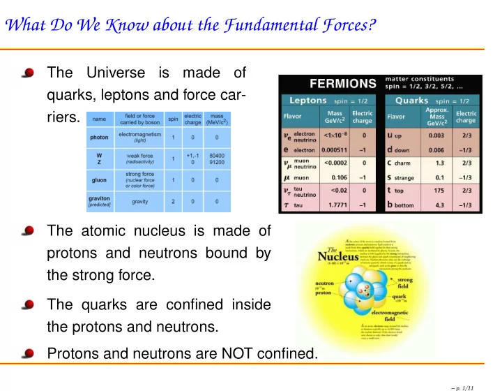
The Universe is made

• f

quarks, leptons and force car- riers. The atomic nucleus is made of protons and neutrons bound by the strong force. The quarks are confined inside the protons and neutrons. Protons and neutrons are NOT confined.

– p. 1/11

The Electric and Magnetic Fields?

d E = ke

dqˆ r r2

The Electric and Magnetic Fields?

d E = ke

dqˆ r r2

d B = km Id

s׈ r r2

– p. 2/11

The Magnetic Field of a Current Loop

Consider a circular loop of radius R located in the y − z plane and carrying a steady current I. What is the magnetic field at an axial point P a distance x from the center of the loop in terms of I, R, x, and any other constants?

x R I P

– p. 3/11

The Magnetic Field of a Current Loop

– p. 4/11

How the Sensor Works - The Hall Effect

– p. 5/11

How the Sensor Works - Electric Current

– p. 6/11

Fitting the Data

fx 2.39 0.298x 5 10 15 20 25 2 4 6 8 10 12 14 x fx

0.27 0.28 0.29 0.3 0.31 0.32 Slope 10 20 30 40 50 60 70 Estimated Variance

In the plot above the value of the y-intercept is kept at its best fit value and the slope is varied. The estimated variance is the following. σ2 = N

i=1(yi − (mxi + b))2

N − d.o.f where N is the number of data points and d.o.f is the number of degrees of freedom (i.e. free parameters) in the fit.

– p. 7/11

Using the Reduced χ2

The χ2 and reduced χ2 are χ2 =

N

• i=1

((yi − f(xi))2 σ2

i

and reduced χ2 = χ2 N − d.o.f where N is the number of data

• points. In Mathematica the estimated

variance is equal to the reduced χ2 if the proper weighting is used.

pA → e+e−X

• R. Muto et al., Evidence for In-Medium Modification of the

φ Meson at Normal Nuclear Density, Phys. Rev. Lett., 98, 042501 (2007).

– p. 8/11

Using the Pasco Hall Probe

– p. 9/11

Biot-Savart Results

Red: Data BlueDashed: Varying n LightBlueSolid: Predicted 0.00 0.05 0.10 0.15 0.20 0.25 0.00000 0.00005 0.00010 0.00015 0.00020 0.00025 rm B T Magnetic Field of a Current Loop

– p. 10/11

Averaging a Data Range in DataStudio

Zoom in on the data range of interest. Click on Selected Statistics in the DataStudio menu bar. Check ‘Min’, ‘Max’, ‘Mean’, and ‘Standard Deviation’. Click and drag to high- light the points of inter-

• est. The results will be

displayed in a box on the plot. To change the output format in the statistics box, (1) Double click on the data set listing (see ‘Data’ window

• n

the left), (2) choose the ‘Nu- meric’ tab and (3) modify the ‘Style’ menu to suit.

Selected Statistics Double click to format statistics – p. 11/11