Week 07 Lectures Signature-based Selection Indexing with Signatures - - PDF document

Week 07 Lectures

Signature-based Selection

Indexing with Signatures

2/103

Signature-based indexing: designed for pmr queries (conjunction of equalities) does not try to achieve better than O(n) performance attempts to provide an "efficient" linear scan Each tuple is associated with a signature a compact (lossy) descriptor for the tuple formed by combining information from multiple attributes stored in a signature file, parallel to data file Instead of scanning/testing tuples, do pre-filtering via signatures. ... Indexing with Signatures

3/103

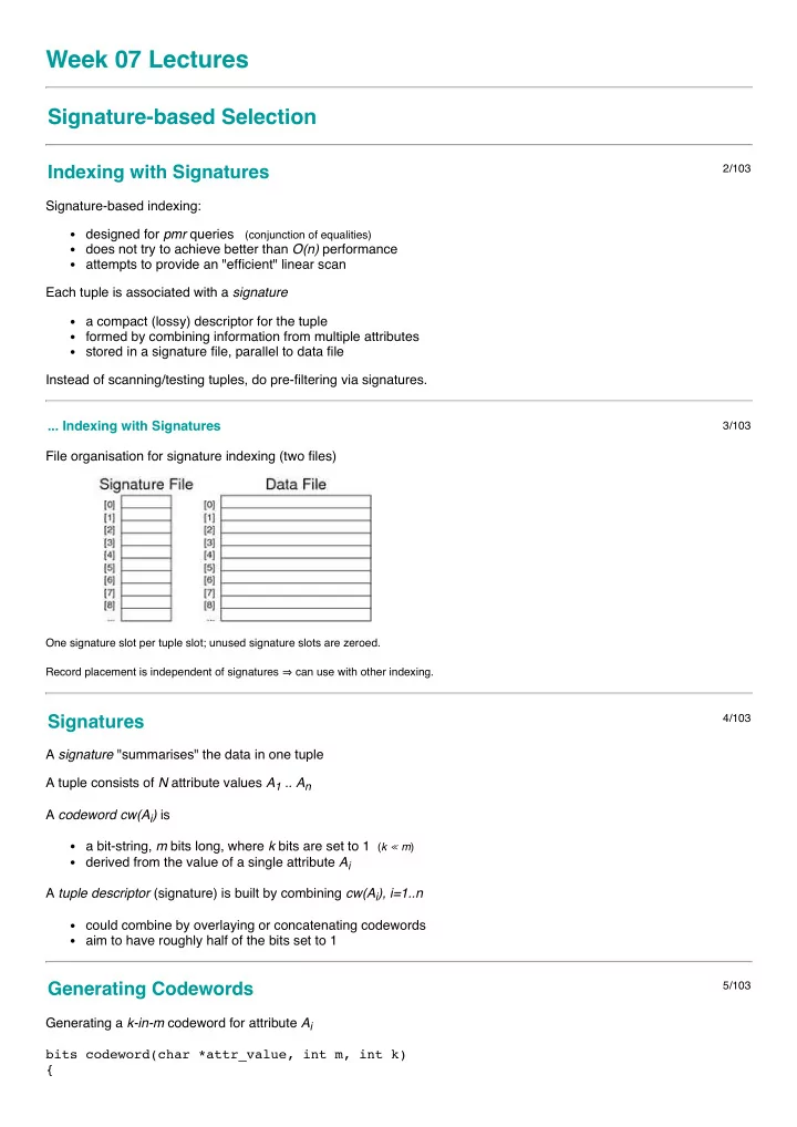
File organisation for signature indexing (two files)

One signature slot per tuple slot; unused signature slots are zeroed. Record placement is independent of signatures ⇒ can use with other indexing.

Signatures

4/103

A signature "summarises" the data in one tuple A tuple consists of N attribute values A1 .. An A codeword cw(Ai) is a bit-string, m bits long, where k bits are set to 1 (k ≪ m) derived from the value of a single attribute Ai A tuple descriptor (signature) is built by combining cw(Ai), i=1..n could combine by overlaying or concatenating codewords aim to have roughly half of the bits set to 1

Generating Codewords

5/103

Generating a k-in-m codeword for attribute Ai bits codeword(char *attr_value, int m, int k) {

int nbits = 0; // count of set bits bits cword = 0; // assuming m <= 32 bits srandom(hash(attr_value)); while (nbits < k) { int i = random() % m; if (((1 << i) & cword) == 0) { cword |= (1 << i); nbits++; } } return cword; // m-bits with k 1-bits and m-k 0-bits }

Superimposed Codewords (SIMC)

6/103

In a superimposed codewords (simc) indexing scheme a tuple descriptor is formed by overlaying attribute codewords A tuple descriptor desc(r) is a bit-string, m bits long, where j ≤ nk bits are set to 1 desc(r) = cw(A1) OR cw(A2) OR ... OR cw(An) Method (assuming all n attributes are used in descriptor): bits desc = 0 for (i = 1; i <= n; i++) { bits cw = codeword(A[i]) desc = desc | cw }

SIMC Example

7/103

Consider the following tuple (from bank deposit database) Branch AcctNo Name Amount Perryridge 102 Hayes 400 It has the following codewords/descriptor (for m = 12, k = 2 ) Ai cw(Ai) Perryridge 010000000001 102 000000000011 Hayes 000001000100 400 000010000100 desc(r) 010011000111

SIMC Queries

8/103

To answer query q in SIMC first generate a query descriptor desc(q) then use the query descriptor to search the signature file desc(q) is formed by OR of codewords for known attributes. E.g. consider the query (Perryridge, ?, ?, ?).

Ai cw(Ai) Perryridge 010000000001 ? 000000000000 ? 000000000000 ? 000000000000 desc(q) 010000000001 ... SIMC Queries

9/103

Once we have a query descriptor, we search the signature file: pagesToCheck = {} for each descriptor D[i] in signature file { if (matches(D[i],desc(q))) { pid = pageOf(tupleID(i)) pagesToCheck = pagesToCheck ∪ pid } } for each P in pagesToCheck { Buf = getPage(f,P) check tuples in Buf for answers } // where ... #define matches(rdesc,qdesc) ((rdesc & qdesc) == qdesc)

Example SIMC Query

10/103

Consider the query and the example database: Signature Deposit Record 010000000001 (Perryridge,?,?,?) 100101001001 (Brighton,217,Green,750) 010011000111 (Perryridge,102,Hayes,400) 101001001001 (Downtown,101,Johnshon,512) 101100000011 (Mianus,215,Smith,700) 010101010101 (Clearview,117,Throggs,295) 100101010011 (Redwood,222,Lindsay,695) Gives two matches: one true match, one false match.

SIMC Parameters

11/103

False match probablity pF = likelihood of a false match How to reduce likelihood of false matches? use different hash function for each attribute (hi for Ai) increase descriptor size (m) choose k so that ≅ half of bits are set Larger m means reading more descriptor data.

Having k too high ⇒ increased overlapping. Having k too low ⇒ increased hash collisions. ... SIMC Parameters

12/103

How to determine "optimal" m and k?

• 1. start by choosing acceptable pF

(e.g. pF ≤ 10-5 i.e. one false match in 10,000)

• 2. then choose m and k to achieve no more than this pF.

Formulae to derive m and k given pF and n: k = 1/loge2 . loge ( 1/pF ) m = ( 1/loge 2 )2 . n . loge ( 1/pF )

Query Cost for SIMC

13/103

Cost to answer pmr query: Costpmr = bD + bq read r descriptors on bD descriptor pages then read bq data pages and check for matches bD = ceil( r/cD ) and cD = floor(B/ceil(m/8)) E.g. m=64, B=8192, r=104 ⇒ cD = 1024, bD=10 bq includes pages with rq matching tuples and rF false matches Expected false matches = rF = (r - rq).pF ≅ r.pF if rq ≪ r E.g. Worst bq = rq+rF, Best bq = 1, Avg bq = ceil(b(rq+rF)/r)

Exercise 1: SIMC Query Cost

14/103

Consider a SIMC-indexed database with the following properties all pages are B = 8192 bytes tuple descriptors have m = 64 bits ( = 8 bytes) total records r = 102,400, records/page c = 100 false match probability pF = 1/1000 answer set has 1000 tuples from 100 pages 90% of false matches occur on data pages with true match 10% of false matches are distributed 1 per page Calculate the total number of pages read in answering the query.

Page-level SIMC

15/103

SIMC has one descriptor per tuple ... potentially inefficient. Alternative approach: one descriptor for each data page. Every attribute of every tuple in page contributes to descriptor. Size of page descriptor (PD) (clearly larger than tuple descriptor): use above formulae but with c.n "attributes" E.g. n = 4, c = 128, pF = 10-3 ⇒ m ≅ 7000bits ≅ 900bytes

Typically, pages are 1..8KB ⇒ 8..64 PD/page (NPD).

Page-Level SIMC Files

16/103

File organisation for page-level superimposed codeword index

Exercise 2: Page-level SIMC Query Cost

17/103

Consider a SIMC-indexed database with the following properties all pages are B = 8192 bytes page descriptors have m = 4096 bits ( = 512 bytes) total records r = 102,400, records/page c = 100 false match probability pF = 1/1000 answer set has 1000 tuples from 100 pages 90% of false matches occur on data pages with true match 10% of false matches are distributed 1 per page Calculate the total number of pages read in answering the query. ... Page-Level SIMC Files

18/103

Improvement: store b m-bit page descriptors as m b-bit "bit-slices" ... Page-Level SIMC Files

19/103

At query time matches = ~0 //all ones for each bit i set to 1 in desc(q) { slice = fetch bit-slice i matches = matches & slice } for each bit i set to 1 in matches { fetch page i

scan page for matching records } Effective because desc(q) typically has less than half bits set to 1

Exercise 3: Bit-sliced SIMC Query Cost

20/103

Consider a SIMC-indexed database with the following properties all pages are B = 8192 bytes r = 102,400, c = 100, b = 1024 page descriptors have m = 4096 bits ( = 512 bytes) bit-slices have b = 1024 bits ( = 128 bytes) false match probability pF = 1/1000 query descriptor has k = 10 bits set to 1 answer set has 1000 tuples from 100 pages 90% of false matches occur on data pages with true match 10% of false matches are distributed 1 per page Calculate the total number of pages read in answering the query.

Similarity Retrieval

Similarity Selection

22/103

Relational selection is based on a boolean condition C evaluate C for each tuple t if C(t) is true, add t to result set if C(t) is false, t is not part of solution result is a set of tuples { t1, t2, ..., tn } all of which satisfy C Uses for relational selection: precise matching on structured data using individual attributes with known, exact values ... Similarity Selection

23/103

Similarity selection is used in contexts where cannot define a precise matching condition can define a measure d of "distance" between tuples d=0 is an exact match, d>0 is less accurate match result is a list of pairs [ (t1,d1), (t2,d2), ..., (tn,dn) ] (ordered by di) Uses for similarity matching: text or multimedia (image/music) retrieval ranked queries in conventional databases

Similarity-based Retrieval

24/103

Similarity-based retrieval typically works as follows: query is given as a query object q (e.g. sample image) system finds objects that are like q (i.e. small distance) The system can measure distance between any object and q ... How to restrict solution set to only the "most similar" objects:

threshold dmax (only objects t such that dist(t,q) ≤ dmax) count k (k closest objects (k nearest neighbours)) ... Similarity-based Retrieval

25/103

Tuple structure for storing such data typically contains id to uniquely identify object (e.g. PostgreSQL oid) metadata (e.g. artist, title, genre, date taken, ...) value of object itself (e.g. PostgreSQL BLOB or bytea) Properties of typical distance functions (on objects x,y,z) dist(x,y) ≥ 0, dist(x,x) = 0, dist(x,y) = dist(y,x) dist(x,z) < dist(x,y) + dist(y,z) (triangle inequality) Distance calculation often requires substantial computational effort ... Similarity-based Retrieval

26/103

Naive approach to similarity-based retrieval q = ... // query object dmax = ... // dmax > 0 => using threshold knn = ... // knn > 0 => using nearest-neighbours Dists = [] // empty list foreach tuple t in R { d = dist(t.val, q) insert (t.oid,d) into Dists // sorted on d } n = 0; Results = [] foreach (i,d) in Dists { if (dmax > 0 && d > dmax) break; if (knn > 0 && ++n > knn) break; insert (i,d) into Results // sorted on d } return Results; Cost = read all r feature vectors + compute distance() for each ... Similarity-based Retrieval

27/103

For some applications, Cost(dist(x,y)) is comparable to Tr ⇒ computing dist(t.val,q) for every tuple t is infeasible. To improve this aspect: compute feature vector which captures "critical" object properties store feature vectors "in parallel" with objects (cf. signatures) compute distance using feature vectors (not objects) i.e. replace dist(t,tq) by dist'(vec(t),vec(tq)) in previous algorithm. Further optimisation: dimension-reduction to make vectors smaller ... Similarity-based Retrieval

28/103

Content of feature vectors depends on application ... image ... colour histogram (e.g. 100's of values/dimensions) music ... loudness/pitch/tone (e.g. 100's of values/dimensions) text ... term frequencies (e.g. 1000's of values/dimensions) Typically use multiple features, concatenated into single vector.

Feature vectors represent points in a very high-dimensional space. Query: feature vector representing one point in vh-dim space. Answer: list of objects "near to" query object in this space.

Example: Content-based Image Retrieval

29/103

User supplies a description or sample of desired image (features). System returns a ranked list of "matching" images from database. ... Example: Content-based Image Retrieval

30/103

At the SQL level, this might appear as ... // relational matching create view Sunset as select image from MyPhotos where title = 'Pittwater Sunset' and taken = '2012-01-01'; // similarity matching with threshold create view SimilarSunsets as select title, image from MyPhotos where (image ~~ (select * from Sunset)) < 0.05

• rder by (image ~~ (select * from Sunset));

where the (imaginary) ~~ operator measures distance between images. ... Example: Content-based Image Retrieval

31/103

Implementing content-based retrieval requires ... a collection of "pertinent" image features e.g. colour, texture, shape, keywords, ... some way of describing/representing image features typically via a vector of numeric values a distance/similarity measure based on features e.g. Euclidean distance between two vectors dist(x,y) = √( (x1-y1)2 + (x2-y2)2 + ... (xn-yn)2 ) ... Example: Content-based Image Retrieval

32/103

Inputs to content-based similarity-retrieval: a database of r objects (obj1, obj2, ..., objr) plus associated ... r × n-dimensional feature vectors (vobj1, vobj2, ..., vobjr) a query image q with associated n-dimensional vector (vq) a distance measure D(vi,vj) : [0..1) (D=0 → vi=vj)

Outputs from content-based similarity-retrieval: a list of the k nearest objects in the database [a1, a2, ... ak]

• rdered by distance D(va1,vq) ≤ D(va2,vq) ≤ ... ≤ D(vak,vq)

Approaches to kNN Retrieval

33/103

Partition-based use auxiliary data structure to identify candidates space/data-partitioning methods: e.g. k-d-B-tree, R-tree, ... unfortunately, such methods "fail" when #dims > 10..20 absolute upper bound on d before linear scan is best d = 610 Approximation-based use approximating data structure to identify candidates signatures: VA-files projections: iDistance, LSH, MedRank, CurveIX, Pyramid ... Approaches to kNN Retrieval

34/103

Above approaches mostly try to reduce number of objects considered. Other optimisations to make kNN retrieval faster reduce I/O by reducing size of vectors (compression, d-reduction) reduce I/O by placing "similar" records together (clustering) reduce I/O by remembering previous pages (caching) reduce cpu by making distance computation faster

Similarity Retrieval in PostgreSQL

35/103

PostgreSQL has always supported simple "similarity" on strings select * from Students where name like '%oo%'; select * from Students where name ~ '[Ss]mit'; Also provides support for ranked similarity on text values using tsvector data type (stemmed, stopped feature vector for text) using tsquery data type (stemmed, stopped feature vector for strings) using @@ similarity operator ... Similarity Retrieval in PostgreSQL

36/103

Example of PostgreSQL text retrieval: create table Docs ( id integer, title text, body text ); // add column to hold document feature vectors alter table Docs add column features tsvector; update Docs set features = to_tsvector('english', title||' '||body); // ask query and get results in ranked order select title, ts_rank(d.features, query) as rank from Docs d, to_tsquery('potter|(roger&rabbit)') as query where query @@ d.features

• rder by rank desc

limit 10; For more details, see PostgreSQL documentation, Chapter 12.

Implementing Join

Join

38/103

DBMSs are engines to store, combine and filter information. Join (⋈) is the primary means of combining information. Join is important and potentially expensive Most common join condition: equijoin, e.g. (R.pk = S.fk) Join varieties (natural, inner, outer, semi, anti) all behave similarly. We consider three strategies for implementing join nested loop ... simple, widely applicable, inefficient without buffering sort-merge ... works best if tables are soted on join attributes hash-based ... requires good hash function and sufficient buffering

Join Example

39/103

Consider a university database with the schema: create table Student( id integer primary key, name text, ... ); create table Enrolled( stude integer references Student(id), subj text references Subject(code), ... ); create table Subject( code text primary key, title text, ... ); ... Join Example

40/103

List names of students in all subjects, arranged by subject. SQL query to provide this information: select E.subj, S.name from Student S, Enrolled E where S.id = E.stude

• rder by E.subj, S.name;

And its relational algebra equivalent: Sort[subj] ( Project[subj,name] ( Join[id=stude](Student,Enrolled) ) ) To simplify formulae, we denote Student by S and Enrolled by E ... Join Example

41/103

Some database statistics: Sym Meaning Value rS # student records 20,000 rE # enrollment records 80,000

cS Student records/page 20 cE Enrolled records/page 40 bS # data pages in Student 1,000 bE # data pages in Enrolled 2,000 Also, in cost analyses below, N = number of memory buffers. ... Join Example

42/103

Out = Student ⋈ Enrolled relation statistics: Sym Meaning Value rOut # tuples in result 80,000 COut result records/page 80 bOut # data pages in result 1,000 Notes: rOut ... one result tuple for each Enrolled tuple COut ... result tuples have only subj and name in analyses, ignore cost of writing result ... same in all methods

Nested Loop Join

Nested Loop Join

44/103

Basic strategy (R.a ⋈ S.b): Result = {} for each page i in R { pageR = getPage(R,i) for each page j in S { pageS = getPage(S,j) for each pair of tuples tR,tS from pageR,pageS { if (tR.a == tS.b) Result = Result ∪ (tR:tS) } } } Needs input buffers for R and S, output buffer for "joined" tuples Terminology: R is outer relation, S is inner relation Cost = bR . bS ... ouch!

Block Nested Loop Join

45/103

Method (for N memory buffers): read N-2-page chunk of R into memory buffers for each S page check join condition on all (tR,tS) pairs in buffers repeat for all N-2-page chunks of R

... Block Nested Loop Join

46/103

Best-case scenario: bR ≤ N-2 read bR pages of relation R into buffers while R is buffered, read bS pages of S Cost = bR + bS Typical-case scenario: bR > N-2 read ceil(bR/N-2) chunks of pages from R for each chunk, read bS pages of S Cost = bR + bS . ceil(bR/N-2) Note: always requires rR.rS checks of the join condition

Exercise 4: Nested Loop Join Cost

47/103

Compute the cost (# pages fetched) of (S ⋈ E) Sym Meaning Value rS # student records 20,000 rE # enrollment records 80,000 cS Student records/page 20 cE Enrolled records/page 40 bS # data pages in Student 1,000 bE # data pages in Enrolled 2,000 for N = 22, 202, 2002 and different inner/outer combinations

Exercise 5: Nested Loop Join Cost (cont)

48/103

If the query in the above example was: select j.code, j.title, s.name from Student s join Enrolled e on (s.id=e.student) join Subject j on (e.subj=j.code) how would this change the previous analysis? What join combinations are there? Assume 2000 subjects, with cJ = 10 How large would the intermediate tuples be? What assumptions?

Compute the cost (# pages fetched, # pages written) for N = 22 ... Block Nested Loop Join

49/103

Why block nested loop join is actually useful in practice ... Many queries have the form select * from R,S where r.i=s.j and r.x=k This would typically be evaluated as Join [i=j] ((Sel[r.x=k](R)), S) If |Sel[r.x=k](R)| is small ⇒ may fit in memory (in small #buffers)

Index Nested Loop Join

50/103

A problem with nested-loop join: needs repeated scans of entire inner relation S If there is an index on S, we can avoid such repeated scanning. Consider Join[R.i=S.j](R,S): for each tuple r in relation R { use index to select tuples from S where s.j = r.i for each selected tuple s from S { add (r,s) to result } } ... Index Nested Loop Join

51/103

This method requires:

• ne scan of R relation (bR)
• nly one buffer needed, since we use R tuple-at-a-time

for each tuple in R (rR), one index lookup on S cost depends on type of index and number of results best case is when each R.i matches few S tuples Cost = bR + rR.SelS (SelS is the cost of performing a select on S). Typical SelS = 1-2 (hashing) .. bq (unclustered index) Trade-off: rR.SelS vs bR.bS, where bR ≪ rR and SelS ≪ bS

Exercise 6: Index Nested Loop Join Cost

52/103

Consider executing Join[i=j](S,T) with the following parameters: rS = 1000, bS = 50, rT = 3000, bT = 600 S.i is primary key, and T has index on T.j T is sorted on T.j, each S tuple joins with 2 T tuples DBMS has N = 12 buffers available for the join Calculate the costs for evaluating the above join using block nested loop join using index nested loop join Costr = # pages read and Costj = # join-condition checks

Sort-Merge Join

Sort-Merge Join

54/103

Basic approach: sort both relations on join attribute (reminder: Join[R.i=S.j](R,S)) scan together using merge to form result (r,s) tuples Advantages: no need to deal with "entire" S relation for each r tuple deal with runs of matching R and S tuples Disadvantages: cost of sorting both relations (already sorted on join key?) some rescanning required when long runs of S tuples ... Sort-Merge Join

55/103

Method requires several cursors to scan sorted relations: r = current record in R relation s = start of current run in S relation ss = current record in current run in S relation ... Sort-Merge Join

56/103

Algorithm using query iterators/scanners: Query ri, si; Tuple r,s; ri = startScan("SortedR"); si = startScan("SortedS"); while ((r = nextTuple(ri)) != NULL && (s = nextTuple(si)) != NULL) { // align cursors to start of next common run while (r != NULL && r.i < s.j) r = nextTuple(ri); if (r == NULL) break; while (s != NULL && r.i > s.j) s = nextTuple(si); if (s == NULL) break; // must have (r.i == s.j) here ... ... Sort-Merge Join

57/103

... // remember start of current run in S TupleID startRun = scanCurrent(si)

// scan common run, generating result tuples while (r != NULL && r.i == s.j) { while (s != NULL and s.j == r.i) { addTuple(outbuf, combine(r,s)); if (isFull(outbuf)) { writePage(outf, outp++, outbuf); clearBuf(outbuf); } s = nextTuple(si); } r = nextTuple(ri); setScan(si, startRun); } } ... Sort-Merge Join

58/103

Buffer requirements: for sort phase: as many as possible (remembering that cost is O(logN) ) if insufficient buffers, sorting cost can dominate for merge phase:

• ne output buffer for result
• ne input buffer for relation R

(preferably) enough buffers for longest run in S ... Sort-Merge Join

59/103

Cost of sort-merge join. Step 1: sort each relation (if not already sorted): Cost = 2.bR (1 + logN-1(bR /N)) + 2.bS (1 + logN-1(bS /N)) (where N = number of memory buffers) Step 2: merge sorted relations: if every run of values in S fits completely in buffers, merge requires single scan, Cost = bR + bS if some runs in of values in S are larger than buffers, need to re-scan run for each corresponding value from R

Sort-Merge Join on Example

60/103

Case 1: Join[id=stude](Student,Enrolled) relations are not sorted on id# memory buffers N=32; all runs are of length < 30 Cost = sort(S) + sort(E) + bS + bE = 2bS(1+log31(bS/32)) + 2bE(1+log31(bE/32)) + bS + bE = 2×1000×(1+2) + 2×2000×(1+2) + 1000 + 2000 = 6000 + 12000 + 1000 + 2000 = 21,000 ... Sort-Merge Join on Example

61/103

Case 2: Join[id=stude](Student,Enrolled)

Student and Enrolled already sorted on id# memory buffers N=4 (S input, 2 × E input, output) 5% of the "runs" in E span two pages there are no "runs" in S, since id# is a primary key For the above, no re-scans of E runs are ever needed Cost = 2,000 + 1,000 = 3,000 (regardless of which relation is outer)

Exercise 7: Sort-merge Join Cost

62/103

Consider executing Join[i=j](S,T) with the following parameters: rS = 1000, bS = 50, rT = 3000, bT = 150 S.i is primary key, and T has index on T.j T is sorted on T.j, each S tuple joins with 2 T tuples DBMS has N = 42 buffers available for the join Calculate the cost for evaluating the above join using sort-merge join compute #pages read/written compute #join-condition checks performed

Hash Join

Hash Join

64/103

Basic idea: use hashing as a technique to partition relations to avoid having to consider all pairs of tuples Requires sufficent memory buffers to hold substantial portions of partitions (preferably) to hold largest partition of outer relation Other issues: works only for equijoin R.i=S.j (but this is a common case) susceptible to data skew (or poor hash function) Variations: simple, grace, hybrid.

Simple Hash Join

65/103

Basic approach: hash part of outer relation R into memory buffers (build) scan inner relation S, using hash to search (probe) if R.i=S.j, then h(R.i)=h(S.j) (hash to same buffer)

• nly need to check one memory buffer for each S tuple

repeat until whole of R has been processed No overflows allowed in in-memory hash table works best with uniform hash function can be adversely affected by data/hash skew ... Simple Hash Join

66/103

Data flow:

... Simple Hash Join

67/103

Algorithm for simple hash join Join[R.i=S.j](R,S): for each tuple r in relation R { if (buffer[h(R.i)] is full) { for each tuple s in relation S { for each tuple rr in buffer[h(S.j)] { if ((rr,s) satisfies join condition) { add (rr,s) to result } } } clear all hash table buffers } insert r into buffer[h(R.i)] } # join tests ≤ rS.cR (cf. nested-loop rS.rR) # page reads depends on #buffers N and properties of data/hash.

Exercise 8: Simple Hash Join Cost

68/103

Consider executing Join[i=j](R,S) with the following parameters: rR = 1000, bR = 50, rS = 3000, bS = 150, cRes = 30 R.i is primary key, each R tuple joins with 2 S tuples DBMS has N = 42 buffers available for the join data + hash have uniform distribution Calculate the cost for evaluating the above join using simple hash join compute #pages read/written compute #join-condition checks performed assume that hash table has L=0.75 for each partition

Grace Hash Join

69/103

Basic approach (for R ⋈ S ): partition both relations on join attribute using hashing (h1) load each partition of R into N-buffer hash table (h2) scan through corresponding partition of S to form results repeat until all partitions exhausted For best-case cost (O(bR + bS) ): need ≥ √bR buffers to hold largest partition of outer relation If < √bR buffers or poor hash distribution need to scan some partitions of S multiple times

... Grace Hash Join

70/103

Partition phase (applied to both R and S): ... Grace Hash Join

71/103

Probe/join phase:

The second hash function (h2) simply speeds up the matching process. Without it, would need to scan entire R partition for each record in S partition.

... Grace Hash Join

72/103

Cost of grace hash join: #pages in all partition files of Rel ≅ bRel (maybe slightly more) partition relation R ... Cost = bR.Tr + bR.Tw = 2bR partition relation S ... Cost = bS.Tr + bS.Tw = 2bS probe/join requires one scan of each (partitioned) relation Cost = bR + bS all hashing and comparison occurs in memory ⇒ ≅0 cost Total Cost = 2bR + 2bS + bR + bS = 3 (bR + bS)

Exercise 9: Grace Hash Join Cost

73/103

Consider executing Join[i=j](R,S) with the following parameters: rR = 1000, bR = 50, rS = 3000, bS = 150, cRes = 30 R.i is primary key, each R tuple joins with 2 S tuples DBMS has N = 43 buffers available for the join data + hash have reasonably uniform distribution Calculate the cost for evaluating the above join using Grace hash join compute #pages read/written compute #join-condition checks performed

assume that no R partition is larger than 40 pages

Exercise 10: Grace Hash Join Cost

74/103

Consider executing Join[i=j](R,S) with the following parameters: rR = 1000, bR = 50, rS = 3000, bS = 150, cRes = 30 R.i is primary key, each R tuple joins with 2 S tuples DBMS has N = 42 buffers available for the join data + hash have reasonably uniform distribution Calculate the cost for evaluating the above join using Grace hash join compute #pages read/written compute #join-condition checks performed assume that one R partition has 50 pages, others < 40 pages assume that the corresponding S partition has 30 pages

Hybrid Hash Join

75/103

A variant of grace join if we have √bR < N < bR+2 create k≪N partitions, m in memory, k-m on disk buffers: 1 input, k-m output, p = N-(k-m)-1 for in-memory partitions When we come to scan and partition S relation any tuple with hash in range 0..m-1 can be resolved

• ther tuples are written to one of k partition files for S

Final phase is same as grace join, but with only k partitions. Comparison: grace hash join creates N-1 partitions on disk hybrid hash join creates m (memory) + k (disk) partitions ... Hybrid Hash Join

76/103

First phase of hybrid hash join with m=1 (partitioning R): ... Hybrid Hash Join

77/103

Next phase of hybrid hash join with m=1 (partitioning S):

... Hybrid Hash Join

78/103

Final phase of hybrid hash join with m=1 (finishing join): ... Hybrid Hash Join

79/103

Some observations: with k partitions, each partition has expected size bR/k holding m partitions in memory needs ⌈mbR/k⌉ buffers trade-off between in-memory partition space and #partitions Best-cost scenario: m = 1, k ≅ ⌈bR/N⌉ (satisfying above constraint) Other notes: if N = bR+2, using block nested loop join is simpler cost depends on N (but less than grace hash join)

Exercise 11: Hybrid Hash Join Cost

80/103

Consider executing Join[i=j](R,S) with the following parameters: rR = 1000, bR = 50, rS = 3000, bS = 150, cRes = 30 R.i is primary key, each R tuple joins with 2 S tuples DBMS has N = 42 buffers available for the join data + hash have reasonably uniform distribution Calculate the cost for evaluating the above join using hybrid hash join with m=1, p=40 compute #pages read/written compute #join-condition checks performed assume that no R partition is larger than 40 pages

Join Summary

81/103

No single join algorithm is superior in some overall sense. Which algorithm is best for a given query depends on: sizes of relations being joined, size of buffer pool any indexing on relations, whether relations are sorted which attributes and operations are used in the query number of tuples in S matching each tuple in R distribution of data values (uniform, skew, ...) Choosing the "best" join algorithm is critical because the cost difference between best and worst case can be very large. E.g. Join[id=stude](Student,Enrolled): 3,000 ... 2,000,000

Join in PostgreSQL

82/103

Join implementations are under: src/backend/executor PostgreSQL suports three kinds of join: nested loop join (nodeNestloop.c) sort-merge join (nodeMergejoin.c) hash join (nodeHashjoin.c) (hybrid hash join) Query optimiser chooses appropriate join, by considering physical characteristics of tables being joined estimated selectivity (likely number of result tuples)

Exercise 12: Outer Join?

83/103

Above discussion was all in terms of theta inner-join. How would the algorithms above adapt to outer join? Consider the following ... select * from R left outer join S on (R.i = S.j) select * from R right outer join S on (R.i = S.j) select * from R full outer join S on (R.i = S.j)

Query Evaluation

Query Evaluation

85/103

... Query Evaluation

86/103

A query in SQL: states what kind of answers are required (declarative) does not say how they should be computed (procedural) A query evaluator/processor : takes declarative description of query (in SQL) parses query to internal representation (relational algebra) determines plan for answering query (expressed as DBMS ops) executes method via DBMS engine (to produce result tuples) Some DBMSs can save query plans for later re-use. ... Query Evaluation

87/103

Internals of the query evaluation "black-box": ... Query Evaluation

88/103

DBMSs provide several "flavours" of each RA operation. For example: several "versions" of selection (σ) are available each version is effective for a particular kind of selection, e.g select * from R where id = 100 -- hashing select * from S -- Btree index where age > 18 and age < 35 select * from T -- MALH file where a = 1 and b = 'a' and c = 1.4 Similarly, π and ⋈ have versions to match specific query types.

... Query Evaluation

89/103

We call these specialised version of RA operations RelOps. One major task of the query processor: given a set of RA operations to be executed find a combination of RelOps to do this efficiently Requires the query translator/optimiser to consider information about relations (e.g. sizes, primary keys, ...) information about operations (e.g. selection reduces size) RelOps are realised at execution time as a collection of inter-communicating nodes communicating either via pipelines or temporary relations

Terminology Variations

90/103

Relational algebra expression of SQL query intermediate query representation logical query plan Execution plan as collection of RelOps query evaluation plan query execution plan physical query plan Representation of RA operators and expressions σ = Select = Sel, π = Project = Proj R ⋈ S = R Join S = Join(R,S), ∧ = &, ∨ = |

Query Translation

91/103

Query translation: SQL statement text → RA expression

Query Translation

92/103

Translation step: SQL text → RA expression Example: SQL: select name from Students where id=7654321;

• - is translated to

RA: Proj[name](Sel[id=7654321]Students)

Processes: lexer/parser, mapping rules, rewriting rules. Mapping from SQL to RA may include some optimisations, e.g.

select * from Students where id = 54321 and age > 50;

• - is translated to

Sel[age>50](Sel[id=54321]Students)

• - rather than ... because of index on id

Sel[id=54321&age>50](Students)

Parsing SQL

93/103

Parsing task is similar to that for programming languages. Language elements: keywords: create, select, from, where, ... identifiers: Students, name, id, CourseCode, ...

• perators: +, -, =, <, >, AND, OR, NOT, IN, ...

constants: 'abc', 123, 3.1, '01-jan-1970', ... PostgreSQL parser ... implemented via lex/yacc (src/backend/parser) maps all identifiers to lower-case (A-Z → a-z) needs to handle user-extendable operator set makes extensive use of catalog (src/backend/catalog)

Mapping SQL to Relational Algebra

94/103

A given SQL query typically has many translations to RA. For example: SELECT s.name, e.subj FROM Students s, Enrolments e WHERE s.id = e.sid AND e.mark < 50; is equivalent to any of πs.name,e.subj( σs.id=e.sid ∧ e.mark<50 ( Students × Enrolments ) ) πs.name,e.subj( σs.id=e.sid ( σe.mark<50 ( Students × Enrolments ) ) ) πs.name,e.subj( σe.mark<50 ( Students ⋈s.id=e.sid Enrolments ) ) ) πs.name,e.subj( Students ⋈s.id=e.sid ( σe.mark<50 ( Enrolments ) ) ) ... Mapping SQL to Relational Algebra

95/103

More complex example: select distinct s.code from Course c, Subject s, Enrolment e where c.id = e.course and c.subject = s.id group by s.id having count(*) > 100; can be translated to the relational algebra expression Uniq(Proj[code]( GroupSelect[groupSize>100]( GroupBy[s.id] ( Enrolment ⋈ Course ⋈ Subjects )))) ... Mapping SQL to Relational Algebra

96/103

The join operations could be done in two different ways: Note: for a join on n tables, there are potentially O(n!) possible trees The query optimiser aims to find version with lowest total cost.

Mapping Rules

97/103

Mapping from SQL → RA expression requires: a collection of templates, ≥1 for each kind of query a process to match an SQL statement to a template mapping rules for translating matched query into RA May need to apply >1 templates to map whole SQL statement. After mapping, apply rewriting rules to "improve" RA expression convert to equivalent, simpler, more efficient expression Note: PostgreSQL also has user-defined mapping rules (CREATE RULE) ... Mapping Rules

98/103

Projection: SELECT a+b AS x, c AS y FROM R ... ⇒ Proj[x←a+b, y←c](R)

SQL projection extends RA projection with renaming and assignment

Join: SELECT ... FROM ... R, S ... WHERE ... R.f op S.g ... , or SELECT ... FROM ... R JOIN S ON (R.f op S.g) ... WHERE ... ⇒ Join[R.f op S.g ](R,S) ... Mapping Rules

99/103

Selection: SELECT ... FROM ... R ... WHERE ... R.f op val ... ⇒ Select[R.f op val](R) SELECT ... FROM ... R ... WHERE ... Cond1,R AND Cond2,R ... ⇒ Select[Cond1,R & Cond2,R](R)

• r

⇒ Select[Cond1,R](Select[Cond2,R](R))

Exercise 13: Mapping OR expressions

100/103

Possible mappings for WHERE expressions with AND are SELECT ... FROM ... R ... WHERE ... X AND Y ... ⇒ Select[X & Y](R) or Select[X](Select[Y](R)) What are possible mappings for SELECT ... FROM ... R ... WHERE ... X OR Y ... Use these to translate: select * from R where (a=1 or a=3) and b < c

Mapping Rules

101/103

Aggregation operators (e.g. MAX, SUM, ...): add as new operators in extended RA

e.g. SELECT MAX(age) FROM ... ⇒ max(Proj[age](...))

Sorting (ORDER BY): add Sort operator into extended RA (e.g. Sort[+name,-age](...)) Duplicate elimination (DISTINCT): add Uniq operator into extended RA (e.g. Uniq(Proj(...))) Grouping (GROUP BY, HAVING): add operators into extended RA (e.g. GroupBy, GroupSelect ) ... Mapping Rules

102/103

View example: assuming Employee(id,name,birthdate,salary)

• - view definition

create view OldEmps as select * from Employees where birthdate < '01-01-1960';

• - view usage

select name from OldEmps; yields OldEmps = Select[birthdate<'01-01-1960'](Employees) Projname(OldEmps) ⇒ Projname(Select[birthdate<'01-01-1960'](Employees))

Exercise 14: Mapping Views

103/103

Given the following definitions: create table R(a integer, b integer, c integer); create view RR(f,g,h) as select * from R where a > 5 and b = c; Show how the following might be mapped to RA: select * from RR where f > 10;

Produced: 6 Sep 2018