Week 06 Lectures 1/102 Recap on Implementing Selection Selection = - - PDF document

30/8/18, 10(32 pm Week 06 Lectures Page 1 of 32 file:///Users/jas/srvr/apps/cs9315/18s2/lectures/week06/notes.html

Week 06 Lectures

Recap on Implementing Selection

1/102

Selection = select * from R where C yields a subset of R tuples satisfying condition C a very important (frequent) operation in relational databases Types of selection determined by type of condition

• ne: select * from R where id=k

pmr: select * from R where age=65 rng: select * from R where age≥18 and age≤21 Strategies for implementing selection efficiently arrangement of tuples in file (e.g. sorting, hashing) auxiliary data structures (e.g. indexes, signatures)

Linear Hashing

2/102

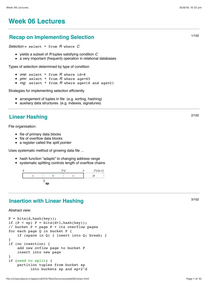
File organisation: file of primary data blocks file of overflow data blocks a register called the split pointer Uses systematic method of growing data file ... hash function "adapts" to changing address range systematic splitting controls length of overflow chains

Insertion with Linear Hashing

3/102

Abstract view: P = bits(d,hash(key)); if (P < sp) P = bits(d+1,hash(key)); // bucket P = page P + its overflow pages for each page Q in bucket P { if (space in Q) { insert into Q; break; } } if (no insertion) { add new ovflow page to bucket P insert into new page } if (need to split) { partition tuples from bucket sp into buckets sp and sp+2^d

30/8/18, 10(32 pm Week 06 Lectures Page 2 of 32 file:///Users/jas/srvr/apps/cs9315/18s2/lectures/week06/notes.html

sp++; if (sp == 2^d) { d++; sp = 0; } } ... Insertion with Linear Hashing

4/102

Splitting block sp=01: ... Insertion with Linear Hashing

5/102

Splitting algorithm:

// partitions tuples between two buckets newp = sp + 2^d; oldp = sp; buf = getPage(f,sp); clear(oldBuf); clear(newBuf); // start filling data page buffers for (i = 0; i < nTuples(buf); i++) { tup = getTuple(buf,i); p = bits(d+1,hash(tup.k)); if (p == newp) addTuple(newBuf,tup); else addTuple(oldBuf,tup); } ... remove and re-insert tuples from ovflow chain ... sp++; if (sp == 2^d) { d++; sp = 0; }

Insertion Cost

6/102

If no split required, cost same as for standard hashing: Costinsert = Best: 1r + 1w, Worst: (1+max(Ov))r + 2w If split occurs, incur Costinsert plus cost of splitting: read block sp (plus all of its overflow blocks) write block sp (and its new overflow blocks) write block sp+2d (and its new overflow blocks) On average, Costsplit = (1+Ov)r + (2+Ov)w

30/8/18, 10(32 pm Week 06 Lectures Page 3 of 32 file:///Users/jas/srvr/apps/cs9315/18s2/lectures/week06/notes.html

Deletion with Linear Hashing

7/102

Deletion is similar to ordinary static hash file. But might wish to contract file when enough tuples removed. Rationale: r shrinks, b stays large ⇒ wasted space. Method: remove last bucket in data file (contracts linearly). Involves a coalesce procedure which is an inverse split.

Hash Files in PostgreSQL

8/102

PostgreSQL uses linear hashing on tables which have been: create index Ix on R using hash (k); Hash file implementation: backend/access/hash hashfunc.c ... a family of hash functions hashinsert.c ... insert, with overflows hashpage.c ... utilities + splitting hashsearch.c ... iterator for hash files

Based on "A New Hashing Package for Unix", Margo Seltzer, Winter Usenix 1991

... Hash Files in PostgreSQL

9/102

PostgreSQL uses a different file organisation ... has a single file containing main and overflow pages has groups of size 2n of data pages in between groups, arbitrary number of overflow pages maintains collection of group pointers in header page each group pointer indicates start of data page group Also maintain a split pointer for data pages. If overflow pages become empty, add to free list and re-use. ... Hash Files in PostgreSQL

10/102

PostgreSQL hash file structure:

30/8/18, 10(32 pm Week 06 Lectures Page 4 of 32 file:///Users/jas/srvr/apps/cs9315/18s2/lectures/week06/notes.html

... Hash Files in PostgreSQL

11/102

Converting bucket # to page address (adapted from pgsql source): typedef unsigned int Word; // which page is primary page of bucket B Word bucket_to_page(Word splits[], B) { Word chunk, base, offset; chunk = (B<2) ? 0 : lg2(B+1)-1; base = splits[chunk];

• ffset = (B<2) ? B : B-(1<<chunk);

return (base + offset); } // returns ceil(log_2(n)) int lg2(Word n) { int i, v; for (i = 0, v = 1; v < n; v <= 1) i++; return i; }

Indexing

12/102

An index is a table/file of (keyVal,tupleID) pairs, e.g.

Indexes

13/102

A 1-d index is based on the value of a single attribute A. Some possible properties of A:

30/8/18, 10(32 pm Week 06 Lectures Page 5 of 32 file:///Users/jas/srvr/apps/cs9315/18s2/lectures/week06/notes.html

may be used to sort data file (or may be sorted on some other field) values may be unique (or there may be multiple instances) Taxonomy of index types, based on properties of index attribute: primary index on unique field, may be sorted on A clustering index on non-unique field, file sorted on A secondary file not sorted on A A given table may have indexes on several attributes. ... Indexes

14/102

Indexes themselves may be structured in several ways: dense

every tuple is referenced by an entry in the index file

sparse

• nly some tuples are referenced by index file entries

single-level

tuples are accessed directly from the index file

multi-level

may need to access several index pages to reach tuple

Index file has total i pages (where typically i ≪ b) Index file has page capacity ci (where typically ci ≫ c) Dense index: i = ceil( r/ci ) Sparse index: i = ceil( b/ci )

Dense Primary Index

15/102

Data file unsorted; one index entry for each tuple

Sparse Primary Index

16/102

30/8/18, 10(32 pm Week 06 Lectures Page 6 of 32 file:///Users/jas/srvr/apps/cs9315/18s2/lectures/week06/notes.html

Data file sorted; one index entry for each page

Exercise 1: Index Storage Overheads

17/102

Consider a relation with the following storage parameters: B = 8192, R = 128, r = 100000 header in data pages: 256 bytes key is integer, data file is sorted on key index entries (keyVal,tupleID): 8 bytes header in index pages: 32 bytes How many pages are needed to hold a dense index? How many pages are needed to hold a sparse index?

Selection with Primary Index

18/102

For one queries: ix = binary search index for entry with key K if nothing found { return NotFound } b = getPage(pageOf(ix.tid)) t = getTuple(b,offsetOf(ix.tid))

• - may require reading overflow pages

return t Worst case: read log2i index pages + read 1+Ov data pages. Thus, Costone,prim = log2 i + 1 + Ov

Assume: index pages are same size as data pages ⇒ same reading cost

... Selection with Primary Index

19/102

For range queries on primary key: use index search to find lower bound read index sequentially until reach upper bound accumulate set of buckets to be examined examine each bucket in turn to check for matches For pmr queries involving primary key:

30/8/18, 10(32 pm Week 06 Lectures Page 7 of 32 file:///Users/jas/srvr/apps/cs9315/18s2/lectures/week06/notes.html

search as if performing one query. For queries not involving primary key, index gives no help.

Exercise 2: Selection with Primary Index

20/102

Consider a range query like select * from R where a between 10 and 30; Give a detailed algorithm for solving such range queries assume table is indexed on attribute a assume file is not sorted on a assume existence of Set data type:

s=empty(); insert(s, n); foreach elems(s)

assume "the usual" operations on relations:

r = openRelation(name,mode); b=nPages(r); file(r)

assume "the usual" operations on pages:

buf=getPage(f,pid); foreach tuples(buf); pid = next(buf)

Insertion with Primary Index

21/102

Overview: insert tuple into page P find location for new entry in index file // could check whether it already exists insert new index entry (k,tid) into index file // tid = tupleID = (P + offset within page) Problem: order of index entries must be maintained need to avoid overflow pages in index so we need to reorganise index file On average, this requires us to read/write half of index file. Costinsert,prim = (log2i)r + i/2.(1r+1w) + (1+Ov)r + (1+δ)w

Deletion with Primary Index

22/102

Overview: find tuple using index mark tuple as deleted delete index entry for tuple If we delete index entries by marking ... Costdelete,prim = (log2 i + 1 + Ov)r + 2w If we delete index entry by index file reorganisation ... Costdelete,prim = (log2 i + 1 + Ov)r + i/2.(1r+1w) + 1w

30/8/18, 10(32 pm Week 06 Lectures Page 8 of 32 file:///Users/jas/srvr/apps/cs9315/18s2/lectures/week06/notes.html

Clustering Index

23/102

Data file sorted; one index entry for each key value ... Clustering Index

24/102

Index on non-unique ordering attribute Ac. Usually a sparse index; one pointer to first tuple containing value. Assists with: range queries on Ac (find lower bound, then scan data) pmr queries involving Ac (search index for specified value) Insertions are expensive: rearrange index file and data file. Deletions relatively cheap (similar to primary index).

(Note: can't mark index entry for value X until all X tuples are deleted)

Secondary Index

25/102

Generally, dense index on non-unique attribute As data file is not ordered on attribute As index file is ordered on attribute As Problem: multiple tuples with same value for As. A solution: dense index (Ix2) containing just TupleId's sparse index (Ix1) on dense index containing (key,offset) pairs Each offset references an entry in Ix2 ... Secondary Index

26/102

30/8/18, 10(32 pm Week 06 Lectures Page 9 of 32 file:///Users/jas/srvr/apps/cs9315/18s2/lectures/week06/notes.html

Costpmr = Costrange = (log2i + aq2 + bq.(1 + Ov)) Costrange = (log2i + aq1 + aq2 + bq.(1 + Ov))

Insertion/Deletion with Secondary Index

27/102

Insertion: each insert requires three files to be updated potentially costly rearrangement of index files Deletion: use mark-style (tombstone) deletion for data tuples Ix2 entries: can always mark as "deleted" Ix1 entries: mark only after removing last instance for k in Ix2 periodic "vacuum" to reduce storage overhead if many deletions

Multi-level Indexes

28/102

Above Secondary Index used two index files to speed up search by keeping the initial index search relatively quick Ix1 small (depends on number of unique key values) Ix2 larger (depends on amount of repetition of keys) typically, bIx1 ≪ bIx2 Could improve further by making Ix1 sparse, since Ix2 is guaranteed to be ordered in this case, bIx1 = ceil( bIx2 / ci ) if Ix1 becomes too large, add Ix3 and make Ix2 sparse if data file ordered on key, could make Ix3 sparse Ultimately, reduce top-level of index hierarchy to one page. ... Multi-level Indexes

29/102

Example data file with three-levels of index:

30/8/18, 10(32 pm Week 06 Lectures Page 10 of 32 file:///Users/jas/srvr/apps/cs9315/18s2/lectures/week06/notes.html

Assume: not primary key, c = 100, ci = 3

Select with Multi-level Index

30/102

For one query on indexed key field: I = top level index page for level = 1 to d { read index page I search index page for J'th entry where index[J].key <= K < index[J+1].key if J=0 { return NotFound } I = index[J].page }

• - I is now address of data page

search page I and its overflow pages Read d index blocks and 1+Ov data blocks. Thus, Costone,mli = (d + 1 + Ov)r

(Note that d = ceil( logci r ) and ci is large because index entries are small)

B-Trees

31/102

B-trees are MSTs with the properties: they are updated so as to remain balanced each node has at least (n-1)/2 entries in it each tree node occupies an entire disk page B-tree insertion and deletion methods are moderately complicated to describe can be implemented very efficiently Advantages of B-trees over general MSTs better storage utilisation (around 2/3 full) better worst case performance (shallower) ... B-Trees

32/102

Example B-tree (depth=3, n=3):

30/8/18, 10(32 pm Week 06 Lectures Page 11 of 32 file:///Users/jas/srvr/apps/cs9315/18s2/lectures/week06/notes.html

(Note that nodes are pages, with potential for large branching factor, e.g. n=500)

B-Tree Depth

33/102

Depth depends on effective branching factor (i.e. how full nodes are). Simulation studies show typical B-tree nodes are 69% full. Gives load Li = 0.69 × ci and depth of tree ~ ceil( logLi r ). Example: ci=128, Li=88 Level #nodes #keys root 1 87 1 88 7656 2 7744 673728 3 681472 59288064 Note: ci is generally larger than 128 for a real B-tree.

Insertion into B-Trees

34/102

Overview of the method:

• 1. find leaf node and position in node where entry would be stored
• 2. if node is not full, insert entry into appropriate spot
• 3. if node is full, split node into two half-full nodes

and promote middle element to parent

• 4. if parent full, split and promote

Note: if duplicates not allowed and key is found, may stop after step 1.

Example: B-tree Insertion

35/102

Starting from this tree:

30/8/18, 10(32 pm Week 06 Lectures Page 12 of 32 file:///Users/jas/srvr/apps/cs9315/18s2/lectures/week06/notes.html

insert the following keys in the given order 12 15 30 10 ... Example: B-tree Insertion

36/102

... Example: B-tree Insertion

37/102

B-Tree Insertion Cost

38/102

Insertion cost = CosttreeSearch + CosttreeInsert + CostdataInsert Best case: write one page (most of time)

30/8/18, 10(32 pm Week 06 Lectures Page 13 of 32 file:///Users/jas/srvr/apps/cs9315/18s2/lectures/week06/notes.html

traverse from root to leaf read/write data page, write updated leaf Costinsert = Dr + 1w + 1r + 1w Common case: 3 node writes (rearrange 2 leaves + parent) traverse from root to leaf, holding nodes in buffer read/write data page update/write leaf, parent and sibling Costinsert = Dr + 3w + 1r + 1w ... B-Tree Insertion Cost

39/102

Worst case: 2D-1 node writes (propagate to root) traverse from root to leaf, holding nodes in buffers read/write data page update/write leaf, parent and sibling repeat previous step D-1 times Costinsert = Dr + (2D-1)w + 1r + 1w

Selection with B-Trees

40/102

For one queries: N = B-tree root node while (N is not a leaf node) N = scanToFindChild(N,K) TupleID = scanToFindEntry(N,K) access tuple t using TupleID from N Costone = (D + 1)r For range queries (assume sorted on index attribute): search index to find leaf node for Lo for each leaf node entry until Hi found { access tuple t using TupleId from entry } Costrange = (D + bi + bq)r

B-trees in PostgreSQL

41/102

PostgreSQL implements Lehman/Yao-style B-trees. A variant that works effectively in high-concurrency environments. B-tree implementation: backend/access/nbtree nbtree.c ... interface functions (for iterators) nbtsearch.c ... traverse index to find key value

30/8/18, 10(32 pm Week 06 Lectures Page 14 of 32 file:///Users/jas/srvr/apps/cs9315/18s2/lectures/week06/notes.html

nbtinsert.c ... add new entry to B-tree index ... B-trees in PostgreSQL

42/102

Interface functions for B-trees // build Btree index on relation Datum btbuild(rel,index,...) // insert index entry into Btree Datum btinsert(rel,key,tupleid,index,...) // start scan on Btree index Datum btbeginscan(rel,key,scandesc,...) // get next tuple in a scan Datum btgettuple(scandesc,scandir,...) // close down a scan Datum btendscan(scandesc)

N-dimensional Selection

N-dimensional Queries

44/102

Have looked at one-dimensional queries, e.g. select * from R where a = K select * from R where a between Lo and Hi and heaps, hashing, indexing as ways of efficient implementation. Now consider techniques for efficient multi-dimensional queries. Compared to 1-d queries, multi-dimensional queries typically produce fewer results require us to consider more information require more effort to produce results

Operations for Nd Select

45/102

N-dimensional select queries = condition on ≥1 attributes. pmr = partial-match retrieval (equality tests), e.g. select * from Employees where job = 'Manager' and gender = 'M'; space = tuple-space queries (range tests), e.g. select * from Employees where 20 ≤ age ≤ 50 and 40K ≤ salary ≤ 60K

N-d Selection via Heaps

46/102

30/8/18, 10(32 pm Week 06 Lectures Page 15 of 32 file:///Users/jas/srvr/apps/cs9315/18s2/lectures/week06/notes.html

Heap files can handle pmr or space using standard method: // select * from R where C r = openRelation("R",READ); for (p = 0; p < nPages(r); p++) { buf = getPage(file(r), p); for (i = 0; i < nTuples(buf); i++) { t = getTuple(buf,i); if (matches(t,C)) add t to result set } } Costpmr = Costspace = b

N-d Selection via Multiple Indexes

47/102

DBMSs already support building multiple indexes on a table. Which indexes to build depends on which queries are asked. create table R (a int, b int, c int); create index Rax on R (a); create index Rbx on R (b); create index Rcx on R (c); create index Rabx on R (a,b); create index Racx on R (a,c); create index Rbcx on R (b,c); create index Rallx on R (a,b,c); But more indexes ⇒ space + update overheads.

N-d Queries and Indexes

48/102

Generalised view of pmr and space queries: select * from R where a1 op1 C1 and ... and an opn Cn pmr : all opi are equality tests. space : some opi are range tests. Possible approaches to handling such queries ...

• 1. use index on one ai to reduce tuple tests
• 2. use indexes on all ai, and intersect answer sets

... N-d Queries and Indexes

49/102

If using just one of several indexes, which one to use? select * from R where a1 op1 C1 and ... and an opn Cn The one with best selectivity for ai opi Ci (i.e. fewest matches) Factors determining selectivity of ai opi Ci

30/8/18, 10(32 pm Week 06 Lectures Page 16 of 32 file:///Users/jas/srvr/apps/cs9315/18s2/lectures/week06/notes.html

assume uniform distribution of values in dom(ai) equality test on primary key gives at most one match equality test on larger dom(ai) ⇒ less matches range test over large part of dom(ai) ⇒ many matches ... N-d Queries and Indexes

50/102

Implementing selection using one of several indices: // Query: select * from R where a1op1C1 and ... and anopnCn // choose ai with best selectivity TupleIDs = IndexLookup(R,ai,opi,Ci) // gives { tid1, tid2, ...} for tuples satisfying aiopiCi PageIDs = { } foreach tid in TupleIDs { PageIDs = PageIDs ∪ {pageOf(tid)} } // PageIDs = a set of bqix page numbers ... Cost = Costindex + bqix (some pages do not contain answers, bqix > bq)

DBMSs typically maintain statistics to assist with determining selectivity

... N-d Queries and Indexes

51/102

Implementing selection using multiple indices: // Query: select * from R where a1op1C1 and ... and anopnCn // assumes an index on at least ai TupleIDs = IndexLookup(R,a1,op1,C1) foreach attribute ai with an index { tids = IndexLookup(R,ai,opi,Ci) TupleIDs = TupleIDs ∩ tids } PageIDs = { } foreach tid in TupleIDs { PageIDs = PageIDs ∪ {pageOf(tid)} } // PageIDs = a set of bq page numbers ... Cost = k.Costindex + bq (assuming indexes on k of n attrs)

Exercise 3: One vs Multiple Indices

52/102

Consider a relation with r = 100,000, B = 4K, defined as: create table Students ( id integer primary key, name char(10), -- simplified gender char(1) -- 'm' or 'f', birthday date -- 1980 .. 2000 ); ... and a query on this relation ...

30/8/18, 10(32 pm Week 06 Lectures Page 17 of 32 file:///Users/jas/srvr/apps/cs9315/18s2/lectures/week06/notes.html

select * from Students where gender='m' and birthday='YYYY-02-29' which has a B-tree index on each attribute ... describe the selectivity of each attribute estimate the cost of answering using one index estimate the cost of answering using both indices

Bitmap Indexes

53/102

Alternative index structure, focussing on sets of tuples: Index contains bit-strings of r bits, one for each value/range ... Bitmap Indexes

54/102

Answering queries using bitmap index: Matches = AllOnes(r) foreach attribute A with index { // select ith bit-string for attribute A // based on value associated with A in WHERE Matches = Matches & Bitmaps[A][i] } // Matches contains 1-bit for each matching tuple foreach i in 0..r { if (Matches[i] == 0) continue; t = fetchTuple(i) Results = Results ∪ {t} } ... Bitmap Indexes

55/102

Storage costs for bitmap indexes:

• ne bitmap for each value/range for each indexed attribute

each bitmap has length ceil(r/8) bytes e.g. with 50K records and 8KB pages, bitmap fits in one page Query execution costs for bitmap indexes: read one bitmap for each indexed attribute in query perform bitwise AND on bitmaps (in memory) read pages containing matching tuples

30/8/18, 10(32 pm Week 06 Lectures Page 18 of 32 file:///Users/jas/srvr/apps/cs9315/18s2/lectures/week06/notes.html

Note: bitmaps could index pages (shorter bitmaps, more comparisons)

Exercise 4: Bitmap Index

56/102

Using the following file structure: Show how the following queries would be answered: select * from Parts where colour='red' and price < 4.00 select * from Parts where colour='green' or colour ='blue'

Hashing for N-d Selection

Hashing and pmr

58/102

For a pmr query like select * from R where a1 = C1 and ... and an = Cn if one ai is the hash key, query is very efficient if no ai is the hash key, need to use linear scan Can be alleviated using multi-attribute hashing (mah) form a composite hash value involving all attributes at query time, some components of composite hash are known

(allows us to limit the number of data pages which need to be checked)

MA.hashing works in conjunction with any dynamic hash scheme. ... Hashing and pmr

59/102

Multi-attribute hashing parameters: file size = b = 2d pages ⇒ use d-bit hash values relation has n attributes: a1, a2, ...an attribute ai has hash function hi

30/8/18, 10(32 pm Week 06 Lectures Page 19 of 32 file:///Users/jas/srvr/apps/cs9315/18s2/lectures/week06/notes.html

attribute ai contributes di bits (to the combined hash value) total bits d = ∑i=1n di a choice vector (cv) specifies for all k ... bit j from hi(ai) contributes bit k in combined hash value

MA.Hashing Example

60/102

Consider relation Deposit(branch,acctNo,name,amount) Assume a small data file with 8 main data pages (plus overflows). Hash parameters: d=3 d1=1 d2=1 d3=1 d4=0 Note that we ignore the amount attribute (d4=0) Assumes that nobody will want to ask queries like select * from Deposit where amount=533 Choice vector is designed taking expected queries into account. ... MA.Hashing Example

61/102

Choice vector: This choice vector tells us: bit 0 in hash comes from bit 0 of hash1(a1) ( b1,0 ) bit 1 in hash comes from bit 0 of hash2(a2) ( b2,0 ) bit 2 in hash comes from bit 0 of hash3(a3) ( b3,0 ) bit 3 in hash comes from bit 1 of hash1(a1) ( b1,1 )

• etc. etc. etc. (up to as many bits of hashing as required, e.g. 32)

... MA.Hashing Example

62/102

Consider the tuple: branch acctNo name amount Downtown 101 Johnston 512 Hash value (page address) is computed by:

30/8/18, 10(32 pm Week 06 Lectures Page 20 of 32 file:///Users/jas/srvr/apps/cs9315/18s2/lectures/week06/notes.html

MA.Hashing Hash Functions

63/102

Auxiliary definitions: #define MaxHashSize 32 typedef unsigned int HashVal; // extracts i'th bit from hash value #define bit(i,h) (((h) & (1 << (i))) >> (i)) // choice vector elems typedef struct { int attr, int bit } CVelem; typedef CVelem ChoiceVec[MaxHashSize]; // hash function for individual attributes HashVal hash1(Tuple t, int i) { ... } ... MA.Hashing Hash Functions

64/102

Produce combined d-bit hash value for tuple t: HashVal hash(Tuple t, ChoiceVec cv, int d) { HashVal h[nAttr(t)+1]; // hash for each attr HashVal res = 0, oneBit; int i, a, b; for (i = 1; i <= nAttr(t); i++) h[i] = hash1(t,i); for (i = 0; i < d; i++) { a = cv[i].attr; b = cv[i].bit;

• neBit = bit(b, h[a]);

res = res | (oneBit << i); } return res; }

Exercise 5: Multi-attribute Hashing

65/102

Compute the hash value for the tuple ('John Smith','BSc(CompSci)',1990,99.5) where d=6, d1=3, d2=2, d3=1, and cv = <(1,0), (1,1), (2,0), (3,0), (1,2), (2,1), (3,1), (1,3), ...> hash1('John Smith') = ...0101010110110100 hash2('BSc(CompSci)') = ...1011111101101111 hash3(1990) = ...0001001011000000

Queries with MA.Hashing

66/102

In a partial match query:

30/8/18, 10(32 pm Week 06 Lectures Page 21 of 32 file:///Users/jas/srvr/apps/cs9315/18s2/lectures/week06/notes.html

values of some attributes are known values of other attributes are unknown E.g. select amount from Deposit where branch = 'Brighton' and name = 'Green' for which we use the shorthand (Brighton, ?, Green, ?) ... Queries with MA.Hashing

67/102

In composite hash for query, values for some bits are unknown: What this tells us: any matching tuples must be in pages 101, 111 ... Queries with MA.Hashing

68/102

Consider the query: select amount from Deposit where name = 'Green' Need to check pages: 100, 101, 110, 111.

Exercise 6: Partial hash values in MAH

69/102

Given the following: d=6, b=26, CV = <(0,0),(0,1),(1,0),(2,0),(1,1),(0,2), ...> hash (a) = ...00101101001101 hash (b) = ...00101101001101 hash (c) = ...00101101001101 What are the query hashes for each of the following:

30/8/18, 10(32 pm Week 06 Lectures Page 22 of 32 file:///Users/jas/srvr/apps/cs9315/18s2/lectures/week06/notes.html

(a,b,c), (?,b,c), (a,?,?), (?,?,?)

MA.Hashing Query Algorithm

70/102

// Builds the partial hash value (e.g. 10*0*1) // Treats query like tuple with some attr values missing nstars = 0; for each attribute i in query Q { if (hasValue(Q,i)) { set d[i] bits in composite hash using choice vector and hash(Q,i) } else { set d[i] *'s in composite hash using choice vector nstars++; } } ... ... MA.Hashing Query Algorithm

71/102

... // Use the partial hash to find candidate pages r = openRelation("R",READ); for (i = 0; i < 2**nstars; i++) { P = composite hash replace *'s in P using i and choice vector Buf = readPage(file(r), P); for each tuple T in Buf { if (T satisfies pmr query) add T to results } }

Exercise 7: Representing Stars

72/102

Our hash values are bit-strings (e.g. 0100101110101) MA.Hashing introduces a third value (* = unknown) How could we represent "bit"-strings like 01011*1*0**010?

Exercise 8: MA.Hashing Query Cost

73/102

Consider R(x,y,z) using multi-attribute hashing where d = 9 dx = 5 dy = 3 dz = 1 How many buckets are accessed in answering each query?

• 1. select * from R where x = 4 and y = 2 and z = 1
• 2. select * from R where x = 5 and y = 3
• 3. select * from R where y = 99

30/8/18, 10(32 pm Week 06 Lectures Page 23 of 32 file:///Users/jas/srvr/apps/cs9315/18s2/lectures/week06/notes.html

• 4. select * from R where z = 23
• 5. select * from R where x > 5

Query Cost for MA.Hashing

74/102

Multi-attribute hashing handles a range of query types, e.g. select * from R where a=1 select * from R where d=2 select * from R where b=3 and c=4 select * from R where a=5 and b=6 and c=7 A relation with n attributes has 2n different query types. Different query types have different costs (different no. of *'s) Query distribution gives probability pQ of asking each query type Q. ... Query Cost for MA.Hashing

75/102

For a relation R(a,b,c,d) ... select * from R where a=1

• - has 1 specified attribute (a)
• - has 3 unspecified attributes (b,c,d)

select * from R where b=5 and d=2

• - has 2 specified attributes (b,d)
• - has 2 unspecified attributes (a,c)

select * from R where a=1 and b=5 and c=3 and d=2

• - has 4 specified attributes (a,b,c,d)
• - has 0 unspecified attributes

... Query Cost for MA.Hashing

76/102

Consider a query of type Q with m attributes unspecified. Each unspecified Ai contributes di *'s. Total number of *'s is s = ∑i ∉ Q di. ⇒ Number of pages to read is 2s = ∏i ∉ Q 2di. Ignoring overflows, Cost(Q) = 2s (where s is determined by Q) Including overflows, Cost(Q) = 2s(1+Ov) ... Query Cost for MA.Hashing

77/102

Min query cost occurs when all attributes are used in query Min Costpmr = 1

30/8/18, 10(32 pm Week 06 Lectures Page 24 of 32 file:///Users/jas/srvr/apps/cs9315/18s2/lectures/week06/notes.html

Max query cost occurs when no attributes are specified Max Costpmr = 2d = b Average cost is given by weighted sum over all query types: Avg Costpmr = ∑Q pQ ∏i ∉ Q 2di

Aim to minimise the weighted average query cost over possible query types

Optimising MA.Hashing Cost

78/102

For a given application, useful to minimise Costpmr. Can be achieved by choosing appropriate values for di (cv) Heuristics: distribution of query types (more bits to frequently used attributes) size of attribute domain (≤ #bits to represent all values in domain) discriminatory power (more bits to highly discriminating attributes) Trade-off: making query type Qj more efficient makes Qk less efficient. This is a combinatorial optimisation problem, and can be handled by standard optimisation techniques e.g. simulated annealing.

MA.Hashing Cost Example

79/102

Consider a table with four attributes: (branch, account, name, amount) (abbreviated to (br,ac,nm,amt) ) Possible query types, and likelhood of each: Query type Cost pQ (?, ?, ?, ?) 8 (br, ?, ?, ?) 4 0.25 (?, ac, ?, ?) 4 (br, ac, ?, ?) 2 (?, ?, nm, ?) 4 (br, ?, nm, ?) 2 (?, ac, nm, ?) 2 0.25 (br, ac, nm, ?) 1 (?, ?, ?, amt) 8 (br, ?, ?, amt) 4 (?, ac, ?, amt) 4 (br, ac, ?, amt) 2 (?, ?, nm, amt) 4 (br, ?, nm, amt) 2 0.5

30/8/18, 10(32 pm Week 06 Lectures Page 25 of 32 file:///Users/jas/srvr/apps/cs9315/18s2/lectures/week06/notes.html

(?, ac, nm, amt) 2 (br, ac, nm, amt) 1 Cost values are based on choice vector (dbr = dac = dnm = 1) pQ values can be determined by observation of DB use. ... MA.Hashing Cost Example

80/102

Consider r=106, Nr=100, b=104, d=14. Attribute br occurs in 0.5+0.25 used query types ⇒ allocate many bits to it e.g. d1=6. Attribute nm occurs in 0.5+0.25 of queries ⇒ allocate many bits to it e.g. d3=4. Attribute amt occurs in 0.5 of queries ⇒ allocate less bits to it e.g. d4=2. Attribute ac occurs in 0.25 of queries ⇒ allocate least bits to it e.g. d2=2. ... MA.Hashing Cost Example

81/102

With bits distributed as: d1=6, d2=2, d3=4, d4=2 Query type Cost pQ (br, ?, ?, ?) 28 = 256 0.25 (?, ac, nm, ?) 28 = 256 0.25 (br, ?, nm, amt) 22 = 4 0.5 Cost = 0.5 × 22 + 0.25 × 28 + 0.25 × 28 = 130

Exercise 9: MA.Hashing Design

82/102

Consider relation Person(name,gender,age) with b=32 and ... pQ Query Type Q 0.5 select name from Person where gender=X and age=Y 0.25 select age from Person where name=X 0.25 select name from Person where gender=X Assume that all other query types have pQ=0.

30/8/18, 10(32 pm Week 06 Lectures Page 26 of 32 file:///Users/jas/srvr/apps/cs9315/18s2/lectures/week06/notes.html

Design a choice vector to minimise average selection cost.

Tree Indexes for N-d Selection

Multi-dimensional Tree Indexes

84/102

Over the last 20 years, from a range of problem areas different multi-d tree index schemes have been proposed varying primarily in how they partition tuple-space Consider three popular schemes: kd-trees, Quad-trees, R-trees. Example data for multi-d trees is based on the following relation: create table Rel ( X char(1) check (X between 'a' and 'z'), Y integer check (Y between 0 and 9) ); ... Multi-dimensional Tree Indexes

85/102

Example tuples: Rel('a',1) Rel('a',5) Rel('b',2) Rel('d',1) Rel('d',2) Rel('d',4) Rel('d',8) Rel('g',3) Rel('j',7) Rel('m',1) Rel('r',5) Rel('z',9) The tuple-space for the above tuples:

Exercise 10: Query Types and Tuple Space

86/102

Which part of the tuple-space does each query represent?

Q1: select * from Rel where X = 'd' and Y = 4 Q2: select * from Rel where 'j' < X ≤ 'r' Q3: select * from Rel where X > 'm' and Y > 4 Q4: select * from Rel where 'k' ≤ X ≤ 'p' and 3 ≤ Y ≤ 6

30/8/18, 10(32 pm Week 06 Lectures Page 27 of 32 file:///Users/jas/srvr/apps/cs9315/18s2/lectures/week06/notes.html

kd-Trees

87/102

kd-trees are multi-way search trees where each level of the tree partitions on a different attribute each node contains n-1 key values, pointers to n subtrees ... kd-Trees

88/102

How this tree partitions the tuple space:

Searching in kd-Trees

89/102

// Started by Search(Q, R, 0, kdTreeRoot) Search(Query Q, Relation R, Level L, Node N) { if (isDataPage(N)) { Buf = getPage(fileOf(R),idOf(N))

30/8/18, 10(32 pm Week 06 Lectures Page 28 of 32 file:///Users/jas/srvr/apps/cs9315/18s2/lectures/week06/notes.html

check Buf for matching tuples } else { a = attrLev[L] if (!hasValue(Q,a)) nextNodes = all children of N else { val = getAttr(Q,a) nextNodes = find(N,Q,a,val) } for each C in nextNodes Search(Q, R, L+1, C) } }

Exercise 11: Searching in kd-Trees

90/102

Using the following kd-tree index Answer the queries (m,1), (a,?), (?,1), (?,?)

Quad Trees

91/102

Quad trees use regular, disjoint partitioning of tuple space. for 2d, partition space into quadrants (NW, NE, SW, SE) each quadrant can be further subdivided into four, etc. Example: ... Quad Trees

92/102

Basis for the partitioning: a quadrant that has no sub-partitions is a leaf quadrant each leaf quadrant maps to a single data page subdivide until points in each quadrant fit into one data page

30/8/18, 10(32 pm Week 06 Lectures Page 29 of 32 file:///Users/jas/srvr/apps/cs9315/18s2/lectures/week06/notes.html

ideal: same number of points in each leaf quadrant (balanced) point density varies over space ⇒ different regions require different levels of partitioning this means that the tree is not necessarily balanced Note: effective for d≤5, ok for 6≤d≤10, ineffective for d>10 ... Quad Trees

93/102

The previous partitioning gives this tree structure, e.g.

In this and following examples, we give coords of top-left,bottom-right of a region

Searching in Quad-tree

94/102

Space query example: Need to traverse: red(NW), green(NW,NE,SW,SE), blue(NE,SE).

Exercise 12: Searching in Quad-trees

95/102

Using the following quad-tree index Answer the queries (m,1), (a,?), (?,1), (?,?)

30/8/18, 10(32 pm Week 06 Lectures Page 30 of 32 file:///Users/jas/srvr/apps/cs9315/18s2/lectures/week06/notes.html

R-Trees

96/102

R-trees use a flexible, overlapping partitioning of tuple space. each node in the tree represents a kd hypercube its children represent (possibly overlapping) subregions the child regions do not need to cover the entire parent region Overlap and partial cover means: can optimize space partitioning wrt data distribution so that there are similar numbers of points in each region Aim: height-balanced, partly-full index pages (cf. B-tree) ... R-Trees

97/102

Insertion into R-tree

98/102

Insertion of an object R occurs as follows: start at root, look for children that completely contain R if no child completely contains R, choose one of the children and expand its boundaries so that it does contain R if several children contain R, choose one and proceed to child repeat above containment search in children of current node

• nce we reach data page, insert R if there is room

if no room in data page, replace by two data pages partition existing objects between two data pages update node pointing to data pages

(may cause B-tree-like propagation of node changes up into tree)

Note that R may be a point or a polygon.

Query with R-trees

99/102

Designed to handle space queries and "where-am-I" queries. "Where-am-I" query: find all regions containing a given point P:

30/8/18, 10(32 pm Week 06 Lectures Page 31 of 32 file:///Users/jas/srvr/apps/cs9315/18s2/lectures/week06/notes.html

start at root, select all children whose subregions contain P if there are zero such regions, search finishes with P not found

• therwise, recursively search within node for each subregion
• nce we reach a leaf, we know that region contains P

Space (region) queries are handled in a similar way we traverse down any path that intersects the query region

Exercise 13: Query with R-trees

100/102

Using the following R-tree: Show how the following queries would be answered:

Q1: select * from Rel where X='a' and Y=4 Q2: select * from Rel where X='i' and Y=6 Q3: select * from Rel where 'c'≤X≤'j' and Y=5 Q4: select * from Rel where X='c'

Note: can view unknown value X=? as range min(X) ≤ X ≤ max(X)

Multi-d Trees in PostgreSQL

101/102

Up to version 8.2, PostgreSQL had R-tree implementation Superseded by GiST = Generalized Search Trees GiST indexes parameterise: data type, searching, splitting via seven user-defined functions (e.g. picksplit()) GiST trees have the following structural constraints: every node is at least fraction f full (e.g. 0.5) the root node has at least two children (unless also a leaf) all leaves appear at the same level Details: src/backend/access/gist

Costs of Search in Multi-d Trees

102/102

Difficult to determine cost precisely. Best case: pmr query where all attributes have known values in kd-trees and quad-trees, follow single tree path cost is equal to depth D of tree in R-trees, may follow several paths (overlapping partitions)

30/8/18, 10(32 pm Week 06 Lectures Page 32 of 32 file:///Users/jas/srvr/apps/cs9315/18s2/lectures/week06/notes.html

Typical case: some attributes are unknown or defined by range need to visit multiple sub-trees how many depends on: range, choice-points in tree nodes

Produced: 30 Aug 2018