w 1 h 1 n 1
play

w 1 / h 1 N 1 N 1 w 1 i ... G / h G N 1 N G - PowerPoint PPT Presentation

A Course in Applied Econometrics 1 . The Basic Methodology Lecture 9 : Stratified Sampling Typically, with stratified sampling, some segments of the population are over- or underrepresented by the sampling scheme. If we know Jeff Wooldridge


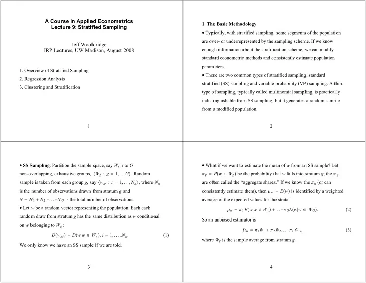
  1. A Course in Applied Econometrics 1 . The Basic Methodology Lecture 9 : Stratified Sampling � Typically, with stratified sampling, some segments of the population are over- or underrepresented by the sampling scheme. If we know Jeff Wooldridge enough information about the stratification scheme, we can modify IRP Lectures, UW Madison, August 2008 standard econometric methods and consistently estimate population parameters. 1. Overview of Stratified Sampling � There are two common types of stratified sampling, standard 2. Regression Analysis stratified (SS) sampling and variable probability (VP) sampling. A third 3. Clustering and Stratification type of sampling, typically called multinomial sampling, is practically indistinguishable from SS sampling, but it generates a random sample from a modified population. 1 2 � SS Sampling : Partition the sample space, say W , into G � What if we want to estimate the mean of w from an SS sample? Let non-overlapping, exhaustive groups, � W g : g � 1,... G � . Random � g � P � w � W g � be the probability that w falls into stratum g ; the � g sample is taken from each group g , say � w gi : i � 1,..., N g � , where N g are often called the “aggregate shares.” If we know the � g (or can consistently estimate them), then � w � E � w � is identified by a weighted is the number of observations drawn from stratum g and N � N 1 � N 2 � ... � N G is the total number of observations. average of the expected values for the strata: � Let w be a random vector representing the population. Each each � w � � 1 E � w | w � W 1 � � ... � � G E � w | w � W G � . (2) random draw from stratum g has the same distribution as w conditional So an unbiased estimator is on w belonging to W g : � w � � 1 w � � 1 � � 2 w � 2 ... � � G w � G , (3) D � w gi � � D � w | w � W g � , i � 1,..., N g . (1) � g is the sample average from stratum g . where w We only know we have an SS sample if we are told. 3 4

  2. � As the strata sample sizes grow, � � Useful to have a formula for � � w is also a consistent estimator of � w as a weighted average across all � w . Also, observations: 2 Var � w � w � � � 1 Var � � 2 Var � w � 1 � � ... � � G � G � . � w � � � 1 / h 1 � N � 1 � N 1 w 1 i � ... � � � G / h G � N � 1 � N G (4) � w Gi � Because Var � w � g � � � g 2 / N g , each of the variances can be estimated in i � 1 i � 1 � N � 1 � N an unbiased fashion by using the usual unbiased variance estimator, � � g i / h g i � w i (7) i � 1 N g 2 � � N g � 1 � � 1 � � � g � w gi � w � g � 2 (5) where h g � N g / N is the fraction of observations in stratum g and in (7) i � 1 we drop the strata index on the observations. and 2 � � 1 � G 2 / N G � 1/2 . se � � � w � � � � 1 2 � 2 / N 1 � ... � � G (6) 5 6 � Variable Probability Sampling : Often used where little, if anything, � Let z i be a G -vector of stratum indicators for draw i , so is known about respondents ahead of time. Still partition the sample p � z i � � p 1 z i 1 � ... � p G z iG (8) space, but an observation is drawn at random. However, if the is the function that delivers the sampling probability for any random observation falls into stratum g , it is kept with (nonzero) sampling draw i . probability, p g . That is, random draw w i is kept with probability p g if � Key assumption for VP sampling: Conditional on being in stratum g , w i � W g . the chance of keeping an observation is p g . Statistically, conditional on � The population is sampled N times (often N is not reported with VP z i (knowing the stratum), s i and w i are independent. Then samples). We always know how many data points were kept; call this E �� s i / p � z i �� w i � � E � w i � . (9) M – a random variable. Let s i be a selection indicator, equal to one if N s i . observation i is kept. So M � � i � 1 7 8

  3. � Equation (9) is the key result for VP sampling. It says that weighting � i � � � / p � z i � where � � � M / N is the fraction of If we define weights as v a selected observation by the inverse of its sampling probability allows observations retained from the sampling scheme, then (11) is us to recover the population mean. Therefore, M � 1 � M � i w i , v (12) N � 1 � N i � 1 � s i / p � z i �� w i (10) i � 1 where only the observed points are included in the sum. � So, can write estimator as a weighted average of the observed data is a consistent estimator of E � w i � . We can also write (10) as � , the observations for stratum g are underpresented in points. If p g � � � M / N � M � 1 � N � s i / p � z i �� w i . (11) the eventual sample (asymptotically), and they receive weight greater i � 1 than one. 9 10 � is obtained from the � SS Sampling: A consistent estimator � 2 . Regression Analysis � Almost any estimation method can be used with SS or VP sampled “weighted” least squares problem data: IV, MLE, quasi-MLE, nonlinear least squares. N b � v i � y i � x i b � 2 , � Linear population model: min (16) i � 1 y � x � � u . (13) where v i � � g i / h g i is the weight for observation i . (Remember, the Two assumptions on u are weighting used here is not to solve any heteroskedasticity problem; it is E � u | x � � 0 to reweight the sample in order to consistently estimate the population (14) parameter � .) E � x � u � � 0 . (15) (15) is enough for consistency, but (14) has important implications for whether or not to weight. 11 12

  4. � Key Question: How can we conduct valid inference using � � ? One Asymptotic variance estimator: � 1 possibility: use the White (1980) “heteroskedasticity-robust” sandwich N � � � g i / h g i � x i � x i estimator. When is this estimator the correct one? If two conditions i � 1 hold: (i) E � y | x � � x � , so that we are actually estimating a conditional N g G � � g / h g � 2 � � � � û gi � x g � û g �� x gi � û gi � x g � û g � � � x gi (18) mean; and (ii) the strata are determined by the explanatory variables, x . g � 1 i � 1 � When the White estimator is not consistent, it is conservative. � 1 N � � � Correct asymptotic variance requires more detailed formulation of the � x i � � g i / h g i � x i . i � 1 estimation problem: N g G � 1 � � � g � y gi � x gi b � 2 min N g . (17) b g � 1 i � 1 13 14 � Usual White estimator ignores the information on the strata of the � One case where there is no gain from subtracting within-strata means is when E � u | x � � 0 and stratification is based on x . observations, which is the same as dropping the within-stratum � If we add the homoskedasticity assumption Var � u | x � � � 2 with � û g . The estimate in (18) is always smaller than the usual averages, x g E � u | x � � 0 and stratification is based on x , the weighted estmator is less White estimate. � Econometrics packages, such as Stata, have survey sampling options efficient than the unweighted estimator. (Both are consistent.) that will compute (18) provided stratum membership is included along with the weights. If only the weights are provided, the larger asymptotic variance is computed. 15 16

  5. � The debate about whether or not to weight centers on two facts: (i) � Analogous results hold for maximum likelihood, quasi-MLE, The efficiency loss of weighting when the population model satisfies nonlinear least squares, instrumental variables. If one knows stratum the classical linear model assumptions and stratification is exogenous. identification along with the weights, the appropriate asymptotic (ii) The failure of the unweighted estimator to consistently estimate � if variance matrix (which subtracts off within-stratum means of the score we only assume of the objective function) is smaller than the form derived by White (1982). For, say, MLE, if the density of y given x is correctly specified, y � x � � u , E � x � u � � 0 , (19) and stratification is based on x , it is better not to weight. (But there are even when stratification is based on x . The weighted estimator cases – including certain treatment effect estimators – where it is consistently estimates � under (19). important to estimate the solution to a misspecified population problem.) 17 18 � Findings for SS sampling have analogs for VP sampling, and some The estimated asymptotic variance in that case is � 1 additional results. First, the Huber-White sandwich matrix applied to M � � x i / p � g i x i the weighted objective function (weighted by the 1/ p g ) is consistent i � 1 when the known p g are used. Second, an asymptotically more efficient M g G � 2 � � � � û gi � x g � û gi � x g � g � û g �� x gi � û g � � � x gi � g � M g / N g , are p (20) estimator is available when the retention frequencies, p g � 1 i � 1 observed, where M g is the number of observed data points in stratum g � 1 M � � � x i / p � g i and N g is the number of times stratum g was sampled. (Is N g known?) x i , i � 1 where M g is the number of observed data points in stratum g . Essentially the same as SS case in (18). 19 20

Download Presentation
Download Policy: The content available on the website is offered to you 'AS IS' for your personal information and use only. It cannot be commercialized, licensed, or distributed on other websites without prior consent from the author. To download a presentation, simply click this link. If you encounter any difficulties during the download process, it's possible that the publisher has removed the file from their server.

Recommend


More recommend