Void fraction measurement using low energy X-rays Giwook Kwon a , - - PDF document

Void fraction measurement using low energy X-rays

Giwook Kwon a, Hyungdae Kim a

aDepartment of Nuclear Engineering, Kyung Hee University, Republic of Korea *Corresponding author: hdkims@khu.ac.kr

• 1. Introduction

Various types of two-phase flow occur in the primary loop during accidents and in the secondary loop during normal operation of light water nuclear power plants (NPPs). For example, rapid depressurization of coolant in the primary loop due to loss of coolant accident results in very complex two-phase flow phenomena. Two-phase flow and heat transfer phenomena always exist in the steam generator and condenser in the secondary system. Therefore, accurate understanding and modeling of two- phase flow phenomena is critical in designing and

• perating various components in NPPs.

Various methods have been developed to measure the void fraction and visualize two-phase flow, including typical flow visualization using visible light, static pressure measurement, pressure drop measurement, local multi-sensor probes including electrical conductance and

• ptical probe, and X-ray method.

Each of these techniques has pros and cons. First, for visible light, there exists significant distortion of the resulting image due to deflection of visible light at the two-phase interface. Static pressure measurement method too much relies on two-phase flow pattern. Pressure drop measurement method could change flow characteristics because it requires an invasive installation

• f the measuring device on the fluid. For methods using

local multi-sensor probes, spatial void fractionation in two-phase flow cannot be obtained because it is a point

• r integral method and interrupting the flow of fluids by

installing devices that interfere with the flow of fluids. Lastly, for X-ray methods, spatial void fraction can be

• btained by measuring entire range of the fluid and does

not interrupt the fluid flow. However, it results radiation shielding and thus relatively expensive. Previous two-phase flow visualization studies using X-ray mainly focused on using high-energy sources of 150 keV or more or using the APS system. However, using low-energy X-rays of less than 50 keV requires much less shielding space and cost, making it easy to move and easy to pursue experiment diversity because of the small size of the experimental device. The objective of this study is to visualize two-phase flow phenomena using a low energy (less than 50 keV) X-ray source and to measure void fraction distribution from obtained image data. To this end, a set of calibration tests is carried out to determine a semi-empirical correlation between grayscale values of obtained images and void fraction. In addition, a simple two-phase flow visualization and void fraction measurement experiment is conducted to verify performance of the developed technique.

• 2. Theory

2.1 X-ray imaging X-rays are attenuated when passing through a substance, and the amount of attenuation depends on its thickness and linear attenuation coefficient. The linear attenuation coefficient, the most important factor of all, is the coefficient of X-rays absorbed per unit length when X-rays pass through a substance. The linear attenuation coefficient depends on the energy of the X-ray and the type of material the X-ray passes through. Generally, solid, liquid has a high linear attenuation coefficient and gas has a low linear attenuation coefficient. And the X- ray with higher energy has a lower linear attenuation

• coefficient. Fluorescent materials in the detector emit

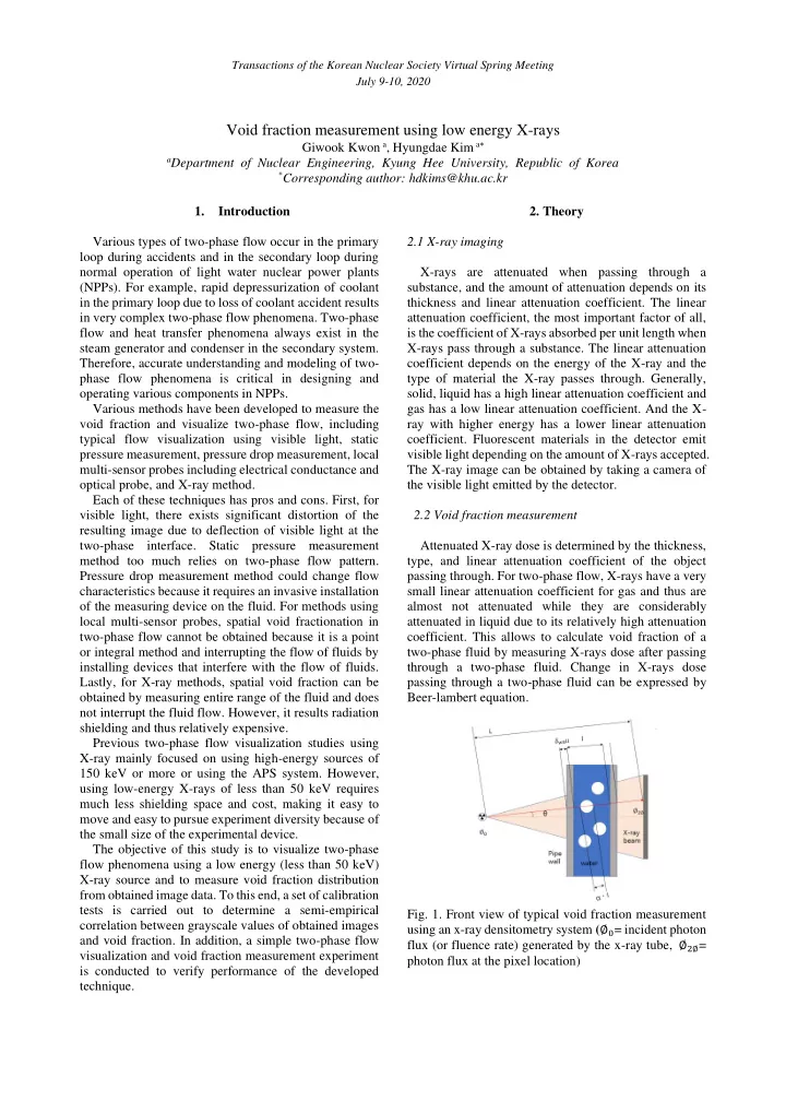
visible light depending on the amount of X-rays accepted. The X-ray image can be obtained by taking a camera of the visible light emitted by the detector. 2.2 Void fraction measurement Attenuated X-ray dose is determined by the thickness, type, and linear attenuation coefficient of the object passing through. For two-phase flow, X-rays have a very small linear attenuation coefficient for gas and thus are almost not attenuated while they are considerably attenuated in liquid due to its relatively high attenuation

• coefficient. This allows to calculate void fraction of a

two-phase fluid by measuring X-rays dose after passing through a two-phase fluid. Change in X-rays dose passing through a two-phase fluid can be expressed by Beer-lambert equation.

• Fig. 1. Front view of typical void fraction measurement

using an x-ray densitometry system (∅0= incident photon flux (or fluence rate) generated by the x-ray tube, ∅2∅= photon flux at the pixel location)

Transactions of the Korean Nuclear Society Virtual Spring Meeting July 9-10, 2020

∅ ̇ 2∅(𝐹, 𝜄) =

∅ ̇ 0(𝐹,𝜄) 𝑀2

∙ 𝑓−[𝛽𝐽(𝜄)∙𝜈𝑕+(1−𝛽)𝐽(𝜄)∙𝜈𝑔+2∙𝜀𝑥𝑏𝑚𝑚(𝜄)∙𝜈𝑞] (1) where α = void fraction, G = grayscale value. However, since measuring ∅ ̇ 𝟑∅(𝐹, 𝜄) is very difficult, the following simplification process is required to convert Eq. (1) into relation between void fraction and grayscale value.

• Limit the measurement range to a pixel and make void

fraction a variable for the length of the fluid.

• Use a square channel to ignore the effects of

attenuation of x-rays depending on the angle.

• Conduct an experiment by keeping X-ray energy

steady and ignoring the variables related to energy.

• The linear attenuation factor of a gas is 10-3 smaller

than that of a fluid or solid, so ignore it. ∅ ̇ 𝟑∅ =

∅ ̇ 𝟏 𝑴𝟑 ∙ 𝒇−[(𝟐−𝜷)𝑱∙𝝂𝒈+𝟑∙𝜺𝒙𝒃𝒎𝒎∙𝝂𝒒]

(2) Therefore, Eq (2) appears. The variables that are constant in Eq (2) are as follows.

• ∅

̇ 𝟏, Because it does not change the release X dose,

• L, it does not change the location of the test object
• 𝜺𝒙𝒃𝒎𝒎 ∙ 𝝂𝒒, does not change the thickness and type of

the test tube's wall.

• I, As the size of the test tube is not changed

If this is integrated into one variable, it becomes Eq. (3). 𝑶 =

∅ ̇ 𝟏 𝑴𝟑 ∙ 𝒇−[𝟑∙𝜺𝒙𝒃𝒎𝒎∙𝝂𝒒+𝑱𝝂𝒈]

(3) When Eq (3) is substituted for Eq. (2) and the left side is converted to a grayscale value, Eq. (4) appears. 𝐇 = 𝐎𝒇𝑱𝝂𝒈𝜷 (4) where 𝑱 = total length of test section = 25 mm, 𝝂𝒈 = linear attenuation coefficient for water at 30 keV = 0.36 cm-1, 𝑱𝝂𝒈 = 0.94, N is the coefficient of the above

• expression. N can be determined by calibration

experiments.

• 3. Calibration

3.1 X-ray imaging setup Experimental design for void fraction correction experiment and two-phase flow visualization are shown in Figure 2. First, the X-ray tube (Oxford's jupiter 5000) provides a stable supply of 50 kvP, 1 mA or less, and is connected to a device that controls voltage and current. The X-ray tube supplies X-rays at a 26˚ angle and has a distance of 660 mm from the X-ray tube and detector.

• Fig. 2. Schematic of experimental setup
• Fig. 3. Schematic of visualization
• Fig. 4. Schematic of measuring void fraction

The experimental

• bject

for two-phase flow photography consists of square acrylic plates 2 mm thick and has an internal diameter of 25 mm. Connect the pump, providing air by drilling a 6mm hole on the bottom. The experimental object for void fraction calibration consists of a triangular acrylic plate 2 mm thick, 120 mm high and 25 mm inner diameter at the bottom, 1 mm inner diameter at the top. The two experimental objects are

Transactions of the Korean Nuclear Society Virtual Spring Meeting July 9-10, 2020

placed in the same position. Detector is the image intensifier of Toshiba and converts the absorbed X-ray into visible light. The visible light emitted by the output window is filmed with an exposure time of 30 fps, 1000 μs using Phantom's high speed camera and transmits the image to the computer. X-rays used a maximum energy

• f 50 keV and a tube current of 1 mA.

3.2 Void fraction calibration

• Fig. 5. Relationship between grayscale value and void

fraction (exposure time = 1000 μs)

The calibration experiment was conducted using a triangular channel. Water of 25 mm in thickness corresponds to the void fraction value of 1. Results analysis used MATLAB 2014a. First, synthesize 90 photos and divide the image of 120 mm experimental device into 10 mm units. This has the effect of dividing the void fraction into 0.09 units. Average the grayscale value of the segmented part pixel using MATLAB. As shown in Figure 5, void fraction and grayscale value draw a graph of the exponential function. And the coefficient of the exponential function is 0.63, which shows an error of 0.94 and 29% of the value of the exponential function coefficient 𝑱𝝂𝒈 of Eq. (4). This can be explained by the error of the energy dependence

• f the linear attenuation factor of the fluid. The values
• btained through the experiment are similar to those
• btained in Eq. (4). This shows that the grayscale value

can act as a significant criterion in measuring void fraction.

• 4. Pre-test for verification
• Fig. 6. Two-phase flow image obtained from X-ray system of

1000 Hz at (a) 300 frame (b) 600 frame (c) 900 frame

• Fig. 7. Void fraction distribution at 1pixel over time

Figure 6 shows serial images of two-phase flow

• btained with the developed X-ray visualization setup.

Figure 6 shows fast bubble’s boundary in the two-phase

• flow. Later, above image might be synthesized and

presented according to time flows. Figure 7 shows temporal variation in void fraction at the single pixel marked at Fig. 6. It shows fluctuation of the two-phase flow.

Transactions of the Korean Nuclear Society Virtual Spring Meeting July 9-10, 2020

• Fig. 8. Void fraction distribution along the pixel location (a)

300 frame (b) 600 frame (c) 900 frame

The corresponding void fraction distribution along the line indicated in the images in Fig. 6 are shown in Fig. 8. The negative void fraction values in the plot are

• unphysical. This is due to the basic pixel error in the

calibration data.

• 5. Conclusion

In the present work, the low-energy X-ray imaging system was developed for high-speed visualization of two-phase flow of water at the frame rate of 1000 Hz and the spatial resolution of 170 m. The setup is small and simple and thus can be applied to various experimental environments. In addition, two-dimensional distribution of void fraction for two-phase flow were measured using the semi-empirical calibration equation. However, some unphysical negative void fraction data were obtained. Those might be caused due to errors in the calibration procedure, which should be reduced by solving basic pixel error in the future work. ACKNOLEDGEMENT This work was supported by the National Research Foundation of Korea(NRF) grant funded by the Korea government(MSIT) (No. 2018M2B2A906584122). REFERENCES [1] Kyle Song and Yang Liu “A compact x-ray system for two-phase flow measurement”, Measurement Scienc e and Techology, Volume 29, 2018 [2] L. Rossi and R. De Fayard and S. Kassab, "Measurements using X‐ray attenuation vertical distribution of the void fraction for different flow regimes in a horizontal pipe", Nuclear Engineering and Design, Voulme 336, 2018, pp 129-140 [3] J. H. Hubbell, "Photon Cross Sections, Attenuation Coefficients, and Energy Absorption Coefficients From 10 keV to 100 GeV”, National Bureau Of Standards , 1969

Transactions of the Korean Nuclear Society Virtual Spring Meeting July 9-10, 2020