
SLIDE 1
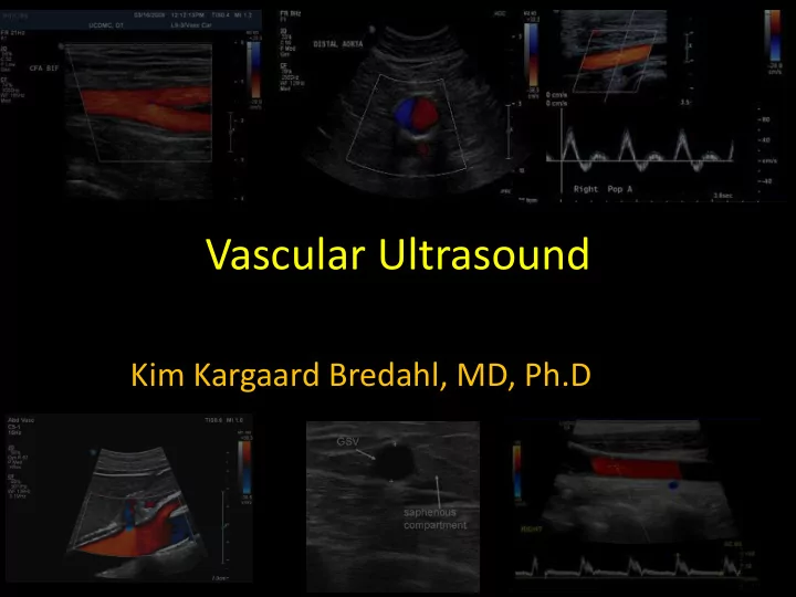
Vascular Ultrasound Kim Kargaard Bredahl, MD, Ph.D Background - - PowerPoint PPT Presentation
Vascular Ultrasound Kim Kargaard Bredahl, MD, Ph.D Background Resident in vascular surgery Vascular ultrasound on a daily basis Stenosis Flow measurement Aneurysms (size) Ph.d thesis 3D and contrast-enhanced ultrasound in
– Stenosis – Flow measurement – Aneurysms (size)
endovascular aneurysm repair surveillance
– Size and flow detection
– Basic course – Advanced course
kimbredahl79@gmail.com
the machinery
Doppler spectrum
related pitfalls
Vascular Surgery: Located on 11th floor, entrance 3, central building.
kimbredahl79@gmail.com
kimbredahl79@gmail.com
Size
Flow detection
for bypass Morphologic and Dynamic flow visualization in human or animals Volume flow
Contrast
thrombus evaluation
Research area
Velocities Flow Pattern
– Can be repeated and is harmless – Dynamic information – Morphology
– Operator dependent
– Bland Altman plots
kimbredahl79@gmail.com
Brightness mode (B- mode) also called grey- scale imaging
Colour Spectral analysis Doppler Ultrasound - Dynamics
CD Player – do you remember it? Receiver Loudspeaker
Amplification Raw data
Transducer Mechanical energy Filtered and amplified Received information Displayed Tissue
Brightness depends on
returning signal called gain
Skin Depth B-mode Two ways to increase signal intensity
reasons is fixed.
level (2D) Amplifier Filter Screen
Mechanical energy Receiving element
Transmitting element
Output power Electric energy Tissue Tissue related
Brightness mode (B-mode)
Brightness mode (B-mode)
Small adjustments to increase the image quality – focal zone Superficial focal zone
ultrasound beam is parallel to the interface
beam is perpendicular to the interface
B-mode
Clear definition of the arterial walls is a good indication of perpendicular position.
kimbredahl79@gmail.com
Heavily calcified arterial Aortic anterior wall Don’t blame the operator
Raw data
Optimal gain level = some echo signal insight the vessel
Adjust the depth of your scanfield
If you can get close it is good ☺
Image resolution Penetration
High-frequency Superficial structures
Low-frequency Deep Structures
From sound to image
Superficial imaging: High frequency low penetration but better image resolution Depth of penetration depend on frequency. Abdominal imaging: Low frequency high penetration – Your neighbour’s bass is more clearly than the treble The lateral image resolution is poorer than the axial image resolution due to higher density of scan lines Linear array 9 MHz 17 MHz 3-5 MHz Curved array Transcranial or cardiac imaging: Large field of view compared to the size of the transducer face. Electronical steering Phased array
Real time biplane imaging Pixels total: Scan field Dimensions are known Pixels outside the segmentation Pixels inside = AAA
kimbredahl79@gmail.com
High-frequency Low-frequency
Handheld Fingercontrol
– Gain
– Depth
– Focus
Brightness mode (B- mode) also called grey- scale imaging
Colour Spectral analysis Doppler Ultrasound - Dynamics
”the Doppler shift”
kimbredahl79@gmail.com
Spectral analysis
Flow towards the transducer will displayed as positive Flow away from the transducer will displayed as negative Tim e
Linear velocity is displayed on the vertical –axis (cm/s) Proportion of blood cells at a particular speed along the third axis – brightness
Vessel
Heart Foot
In this example: Blood flow towards the transducer is coded red Blood flow away from the transducer is coded blue
Colour Doppler
signals in the steering-box
θ
Colour Doppler
Spectral analysis
Flow towards the transducer will displayed as positive Flow away from the transducer will displayed as negative Time
Linear velocity is displayed on the vertical –axis (cm/s) Proportion of blood cells at a particular speed along the third axis – brightness
Vessel
Heart Foot
In this example: Blood flow towards the transducer is coded red Blood flow away from the transducer is coded blue
Colour Doppler
signals in the steering-box
B-mode image
Doppler curve
Velocity is coded Duplex
Colour Doppler
θ
Colour Doppler
SFA External Iliac artery
Remember! The Doppler shift is based on Doppler equation where cosinus function is included, and cosinus to 90 degree is zero
Colour Doppler
1 Cos (θ) Sin (θ)
kimbredahl79@gmail.com
Groin or SFA Poplitea
Colour Doppler
Remember! The pulse repetition frequency is important in
Growth of a tree cannot be observed by watching every second! If the speed is high – you have to watch every second
Low flow PRF too high PRF too low
Peak systolic velocity Mean velocity Framerate
Angle θ
Distance Colour scale Beam path (Steer)
Colour Box
Doppler angle Correction curser Doppler Angle θ Sample Volume
Normal triphasic flow in peripheral artery
Forward and reversed flow are seen simultaneously during the diastolic phase
Reversal flow depends on the peripheral resistance
After exercise
The velocity of blood cells (or Doppler shift freq.) vary with time due to arterial pulsation
Low resistance vessel
kimbredahl79@gmail.com
Normal Triphasic flow After releasing the cuff Normal Triphasic flow Recovery of peripheral resistance
kimbredahl79@gmail.com
superior
kimbredahl79@gmail.com
Blood cells with multiple velocities
Spectral broadening
Laminar or Parabolic flow Disturbed flow Turbulent flow
kimbredahl79@gmail.com
Triphasic signal → Disturbed flow showing spectral broadening → Finally monophasic flow
kimbredahl79@gmail.com
kimbredahl79@gmail.com
– fluid travels faster through the narrow section
x3
Velocity profile in arterial stenosis
Stenotic signal Post-stenotic signal Monofasic signal Tri-phasic signal Blood flow Velocity Decrease in diameter 50% At 70% reduction of diameter a pressure drop
This correspond to a 2-3 fold increase in systolic velocity
kimbredahl79@gmail.com
Linear velocity
D
Flow volume = Cross section . Linear velocity
kimbredahl79@gmail.com
Dist 0.699 cm TAMV 13.8 cm/s Vol Flow 318 mL/ min Area 0.384 cm2
Peak systolic velocity Mean velocity TAMV
kimbredahl79@gmail.com
Related to linear velocity assessment
kimbredahl79@gmail.com
Small sample volume: Reflection only received from fast the fastest moving blood cells Small sample volume: Reflection will be received from all moving blood cells Vol flow = 477 mL / min Vol flow = 318 mL / min
kimbredahl79@gmail.com
fd = f0 – f1 = (2 x V x f0 x cos) / C When calculating the velocity (V) the angle estimation is very important – especially when > 60. Example: Overestimating the angle by 5
Conclusion: Keep the angel < 60 !
30 60 80 10 100 Error in velocity % Degrees
kimbredahl79@gmail.com
High gain → overloading of the instrument → poor direction discrimination Mirror image PSV and TAMV increase Ideal image PSV and TAMV decrease Too low gain → flow may not be detected The ideal gain level
kimbredahl79@gmail.com
The error is 0.084 cm or less than 1 mm. or 11 %
The corresponding failure in vol flow is 21 % going from 459 mL to 362 mL
kimbredahl79@gmail.com
L9-3 MHz L17-5 MHz
Intima No intima For superficial structures take the transducer with the highest frequency available
kimbredahl79@gmail.com
kimbredahl79@gmail.com
Upper LoA =4.7 mm Average 1, 94 mm
kimbredahl79@gmail.com
Diameter forskel Tid 1 sekund Frame rate = 18 By Henrik Sillesen
kimbredahl79@gmail.com
2-6 mm. Difference!
kimbredahl79@gmail.com
Taken the concept of acoustic impedance into account the ideal measurement would be from the most reproducible measurement is from leading edge adventitia
adventitia posterior wall The most reproducible measurement The true volume flow From intima to intima
kimbredahl79@gmail.com
Leading edge
Tunica media Leading edge of adventitia – anterior wall Lumen Grænsen mellem tunica media og tunica adventitia
kimbredahl79@gmail.com
Leading edge of intima Leading edge of adventitia
kimbredahl79@gmail.com
kimbredahl79@gmail.com
Not all vessels are circular Most scanners assume the mean Velocity of sound is 1540 m/s →Systematic underestimation of the Diameter
Medium Speed (C) (m/s) Air 330 Water 1480 Blood 1570 Fat 1450 Muscle 1580 Bone 3500 Soft tissue (average) 1540
kimbredahl79@gmail.com
– Small enough to pass through the capillaries – Large enough to retain in the vascular system
– Completely pulmonary eliminated
Gas SF6 Poor interaction with other molecules Amphophilic shell
Instability → destruction Backscatter = Tissue Signal Low pressure High pressure Oscillation
≠ Tissue signal
– Specific echo signal different from tissue
– Independent from blood flow velocity
– Good safety profile
– 20 gauge cannula – Forward injection in a cubital vein. – 1-2 ml. – Last 6 hours after mixture. – Anti-histamin and adrenalin.
– Diabetic patients
– Plaque size and neovascularization – Thrombus size estimation – Near occlusion / complete occlusion – Flow detection
Microvasculature
Peripheral arterial disease Healthy volunteer Lindner JR, Portland, Oregon. JACC: Cardiovascular imaging 2008
kimbredahl79@gmail.com
– Control colour box
– Pulse repetition frequency
– Spectral analysis
– Extra option ”Walk the Doppler” from CFA to PFA.
Field of view
transducer
analysis
and keep the angle to the Beam path < 60º
Beam path Flow direction
(Keyboard). And your left hand is as important as your right hand.
– Edited by Abigail Thrush and Tim Hartshorne
by contrast-enhanced ultrasound by C. Greis. Clinical
Hemorheology and Microcirculation 49 (2011) 137-149
measurement of peripheral blood flow during exercise in patients with type II diabetes and peripheral artery disease: a systematic review
kimbredahl79@gmail.com
High-frequency Low-frequency
Handheld Fingercontr
CD Player – do you remember it? Receiver Loudspeake r
Amplificatio n Raw data
Transducer Mechanica l energy Filtered and amplified Received informatio n Displaye d Tissue
Raw data
Optimal gain level = some echo signal insight the vessel
Adjust the depth of your scanfield
If you can get close it is good ☺
Brightness mode (B- mode) also called grey- scale imaging
Colour Spectral analysis Doppler Ultrasound - Dynamics
Spectral analysis
Flow towards the transducer will displayed as positive Flow away from the transducer will displayed as negative Tim e
Linear velocity is displayed on the vertical –axis (cm/s) Proportion of blood cells at a particular speed along the third axis – brightness
Vessel
Heart Foot
In this example: Blood flow towards the transducer is coded red Blood flow away from the transducer is coded blue
Colour Doppler
signals in the steering-box
θ
Colour Doppler
SFA External Iliac artery
Remember! The Doppler shift is based on Doppler equation where cosinus function is included, and cosinus to 90 degree is zero
Colour Doppler
1 Cos (θ) Sin (θ)
Colour Doppler
Remember! The pulse repetition frequency is important in
Growth of a tree cannot be observed by watching every second! If the speed is high – you have to watch every second
Low flow PRF too high PRF too low
Peak systolic velocity Mean velocity Framerat e
Angle θ
Distance Colour scale Beam path (Steer)
Colour Box
Doppler angle Correction curser Doppler Angle θ Sample Volume
artery
artery
– Control colour box
– Pulse repetition frequency
– Spectral analysis
– Extra option ”Walk the Doppler” from CFA to PFA.
Field of view
transducer
analysis
and keep the angle to the Beam path < 60º
Beam path Flow direction
(Keyboard). And your left hand is as important as your right hand.
– Displaying the doppler signal – Flow profiles
– Pitfalls
kimbredahl79@gmail.com
– Peripheral blood pressure – Dynamic flow visualization
kimbredahl79@gmail.com
– Morphology
lumen/thrombus
kimbredahl79@gmail.com
– Low flow – Microperfusion
kimbredahl79@gmail.com
Ultrasound = High frequency sound that induces local periodic displacement of particles in the medium
Transducer on Transducer off Displacement Depth
λ
Frequency (f) = 1/τ, number of cycles of displacements during 1 second (Hz). Medical ultrasound scanner typically use frequencies between 2 – 15 MHz
kimbredahl79@gmail.com
Transducer Piezo-electro elements Gel
fd = fr – ft = ( 2 x V x ft x Cos θ) / C
Receiving element Red cells = moving source, Transducer = stationary observer
Transmitting element Transducer = stationary source Red cells = Moving observer. θ : Angle of insonation C: Speed of sound in tissue (1540 m/s) V: Velocity of blood fr: Receiving frequency ft: Transmitted frequency
kimbredahl79@gmail.com
The Doppler signal of flowing blood contains a range of velocities (or Doppler shift frequencies) Bloods cells near the vessel wall will move more slowly
Velocity time
kimbredahl79@gmail.com
Output power Electric energy
Transmitting element
Receiving element
Amplifier Analyser Screen
From sound to image Transducer: Converts energy into another form of energy Ultrasound machine interprets the receiving information
Mechanical energy Vibration
Tissue High-End Frame rate depends on
Reduce field of view. Steady patient! Low-End Two possibilities to increase signal intensity
power, which is
amplification, which is the gain level (2D) but at a certain level signal ≠ noise
kimbredahl79@gmail.com
Skin Brightness proportional to amplitude of echoes – grey scale We assume the speed of ultrasound through the tissue is constant, and we know the generated frequency then we can predict the distance from the source to the reflective boundary
Medium Speed (C) (m/s) Air 330 Water 1480 Blood 1570 Fat 1450 Muscle 1580 Bone 3500 Soft tissue (average) 1540
Depth Distance = (Time . C) / 2
kimbredahl79@gmail.com
Output power Electric energy
Transmitting element
Receiving element
Amplifier Analyser Screen
From sound to image Transducer: Converts energy into another form of energy Ultrasound machine interprets the receiving information
Two possibilities to increase signal intensity
which is often locked
which is the gain level (2D) but at a certain level signal ≠ noise
kimbredahl79@gmail.com
From sound to image
Superficial imaging: Depth of penetration depend on frequency. High frequency low penetration but better image resolution Abdominal imaging: Low frequency high penetration – Your neighbour’s bass is more clearly than the treble The lateral image resolution is poorer the axial image resolution due to higher density of scan lines Linear array 9 MHz 13 MHz 3-5 MHz Curved array Cardiac imaging: Large field of view compared to the size of the transducer face. Electronical steering Phased array
kimbredahl79@gmail.com
Difference in acoustic impedance determines reflection rate
From sound to image – Acoustic impedance: resistance against passage of the sound wave
Similar acoustic impedance
Different acoustic impedance
kimbredahl79@gmail.com
Blood flow towards the transducer is (probably) coded red Blood flow away from the transducer is coded blue
Arterial flow Venous flow
Primarily used for flow detection
θ
Cos (θ) Sin (θ)
Doppler angle θ = 90 then Cos(90) = 0
1
kimbredahl79@gmail.com
kimbredahl79@gmail.com
The Doppler spectrum displays:
Time along the horizontal axis Velocity (Doppler shift) along the vertical axis Proportion of blood cells at a particular speed along the third axis – brightness of the display
Blue The mean velocity Peak systolic velocity
kimbredahl79@gmail.com
Field of view
steering level
kimbredahl79@gmail.com
and keep the angle to the Beam path < 60º
Beam path Flow direction
kimbredahl79@gmail.com
artery
artery
Underestimate the true velocity Align the transducer with reasonable length of the vessel
kimbredahl79@gmail.com
6 PRF too high PRF too low
Aliasing – Flow is going backwards
12 9 3 45 min later 90 min later 135 min later
Especially low flow is not detected
kimbredahl79@gmail.com
artery
artery
B-mode image
Doppler curve
Duplex
kimbredahl79@gmail.com
– Displaying the doppler signal – Flow profiles
kimbredahl79@gmail.com
Colour scale Framerate
Angle θ
Doppler Angle θ Beam path (Steer)
Colour Box
Doppler angle Correction curser Sample Volume Distance Peak systolic velocity Mean velocity
kimbredahl79@gmail.com
Små glatte muskelceller og elastisk fibre Endothelceller Adventitia består mest af kollagen Stor forskel i akustisk impedans fra lav til høj → Refleksion ↑ Måler aldrig IMT på forreste væg
kimbredahl79@gmail.com