Using CP When You Don't Know CP Christian Bessiere LIRMM (CNRS/U. - - PowerPoint PPT Presentation

Using CP When You Don't Know CP

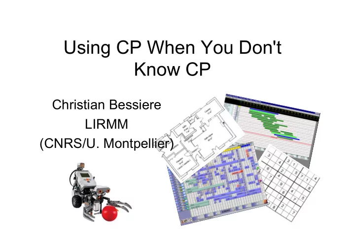
Christian Bessiere LIRMM (CNRS/U. Montpellier)

An illustrative example

5-rooms flat (bedroom, bath, kitchen, sitting, dining) on a 6-room pattern north

• west

north north- east south- east south- west south The pattern:

Constraints of the builder:

– Kitchen and dining must be linked – Bath and kitchen must have a common wall – Bath must be far from sitting – Sitting and dining form a single room

Problem

• How to propose all possible plans?

 a constraint network that encodes the constraints of the builder

Library of constraints

• Constraints :

– X ≠ Y, X = Y – Next(X,Y) = { (nw,n),(nw,sw),(n,nw),(n,ne),(n,s), (ne,n),(ne,se),(sw,nw),(sw,s),(s,sw), (s,n),(s,se),(se,s),(se,ne) } – Far(X,Y) = { (nw,ne),(nw,s),(nw,se),(n,sw),(n,se), (ne,nw),(ne,sw),(ne,s),(sw,n),(sw,ne), (so,se),(s,nw),(s,ne),(se,nw),(se,n),(se,sw) } nw n ne se sw s

A possible viewpoint (variables, domains)

• Variables :

– B (bedroom), – W (washroom), – K (kitchen), – S (sitting), – D (dining)

• Domains : {nw,n,ne,sw,s,se}

nw n ne se sw s

far next next next

A constraint network

Alldiff(K,W,D,S,B) nw,n,ne,sw,s,se

B

nw,n,ne,sw,s,se S nw,n,ne,sw,s,se

D

nw,n,ne,sw,s,se

W

nw,n,ne,sw,s,se

K Bedroom: east Sitting: south Client wishes: K W B S D

a solution

Constraint Programming

Problem Variables Domains Constraints Solution modelling solving

???

Modelling

(“it’s an art, not a science”)

• In the 80s, it was considered as trivial

– Zebra problem (Lewis Carroll) or random problems

• But on “real” problems:

– Which variables ? Which domains ? – Which constraints for encoding the problem?

• And efficiency?

– Which constraints for speeding up the solver?

• Global constraints, symmetries…

 All is in the expertise of the user

If you’re not an expert?

• 1. Choice of variables/domains
• 2. Constraint acquisition
• 3. Improve a basic model

Choice of variables/domains (viewpoints)

• From historical data (former solutions)
• Solutions described in tables (flat data)

D S C W K S D S B K W K S B D

Room Position Dining nw Kitchen n Sitting ne Bedroom sw Wash s Room Position Sitting nw Kitchen n Bedroom ne SàM Wash se Room Position Wash nw Kitchen n Bedroom sw Dining s Sitting se

Extract viewpoints

Room, position Room Position ∅

Room Position Wash nw Kitchen n Bedroom sw Dining s Sitting se

XWash ∈ {nw,n,ne,sw,s,se} XSitting ∈ {nw,n,ne,sw,s,se} ….

Extract viewpoints

• Two viewpoints:

– XB,…,XS ∈ {nw,n,ne,sw,s,se} – Xnw,…,Xse ∈ {W,B,K,D,S,∇}

• Trivial viewpoints:

– X1,…,X5 ∈ {B-nw,B-n,B-sw,…, S-s,S-se} – XB-nw,…,XS-se ∈ {0,1} Room, position Room Position ∅

Room Position wash nw kitchen n bedroom sw dining s sitting se

Connect viewpoints

• VP1: XB,…,XS ∈ {nw,n,ne,sw,s,se}
• VP2: Xnw,…,Xse ∈ {B,W,K,D,S,∇}
• Channelling constraints:

– XB = nw ↔ Xnw = B

“nw” is taken at most once in VP1  alldiff(XB,…,XS) is a constraint in VP1

[like in Law,Lee,Smith07]

Application: sudoku

L1 C4 3 L1 C5 1 L2 C1 3 L2 C3 4 L3 C4 2 L3 C9 8 … … …

L C V XLC=V XLV=C XCV=L Alldiffs learned for free

Connect viewpoints

• We can derive more than just alldiff
• Cardinality constraints can be detected
• Example: a timetabling in which 3 math

courses are given  one of the viewpoints will contain 3 variables representing these 3 courses  In all other viewpoints, we can put a cardinality constraint forcing value “math” to be taken 3 times

If you’re not an expert?

• Choice of variables/domains
• Constraint Acquisition

– Space of networks – Redundancy – Queries

• Improve a basic model

Acquire constraints

• The user doesn’t know how to specify

constraints

• She knows how to discriminate solutions from

non-solutions

– Ex: valid flat vs invalid flat

Use of machine learning techniques

– Interaction by examples (positive e+ or negative e-) – Acquisition of a network describing the problem

Space of possible networks

XD XB XK XW XS ? ? ? ? ? ? ? ?

• Language :

? → { =, ≠, next, far }

• Bias :

XS=XW; next(XS,XB);… …; XK≠XD; far(XK,XD)

Some positive rejected Some negative accepted

Compact SAT encoding

• A SAT formula K representing all

possible networks:

– Each constraint ci

→ a literal bi

– Models(K) = version space – Example e- rejected by {ci,cj,ck}

→ a clause (bi ∨ bj ∨ bk)

– Example e+ rejected by ci

→ a clauses (¬bi)

• m ∈ models(K)

⇒ ϕ(m) = {ci | m(bi)=1} accepts all positive examples and rejects all negative examples

Some negative accepted Some positive rejected

Reduce the space

C(XK,XD): ≠, =, far, next B K W S D e+

1

C(XD,XS): ≠, =, far, next C(XK,XS): ≠, =, far, next e-

2

K W B S D K W S e+

3

B D M e-

4

K W B D S next(XD,XS) ∨ far(XK,XS)

Redundancy

• Constraints are not

independent

• “next(XK,XD) ∧ next(XD,XS) ⇒ far(XK,XS)”
• See local consistencies
• It’s different from attribute-value learning

K M S

Redundancy

• Redundancy prevents convergence

 a set R of redundancy rules:

alldiff(X1,…,Xn) ⇒Xi≠Xj, ∀i,j next(XK,XD) ∧ next(XD,XS) ⇒ far(XK,XS)

• In K we already have:

– next(XD,XS) ∨ far(XK,XS) – next(XK,XD)

• So, from K+R we deduce far(XK,XS)
• Version space = Models(K+R)

– Good properties when R is complete

K M S

Queries

(active learning)

• Examples often lead to little new information (eg,

negative plan with kitchen far from dining)

• The system will propose examples (queries) to speed

up convergence

• Example e rejected by k constraints from the space

– e positive ⇒ k constraints discarded from the space – e negative ⇒ a clause of size k

• Good query = example which reduces the space as

much as possible whatever the answer

Queries

• Negative example e1:

 cle1 = b1∨…∨bk ∈ K+R – find m ∈ models(K+R) such that a single literal bi in cle1 is false – find e2 ∈ sol(ϕ(m)) :

→ e2 violates only constraint ci  bi or ¬bi will go in K

• If sol(ϕ(m))=∅: any conflict-set is a

new redundancy rule  quick convergence

K+R

b1∨…∨bk m contains ¬bi ϕ(m) e2 ∈ sol(ϕ(m)) Query: “e2” ?

An example of constraint acquisition in robotics

(by Mathias Paulin)

• The goal is to automate the burden of

implementing elementary actions of a robot

• Elementary actions are usually

implemented by hand by engineers (complex physic laws, kinetic momentum, derivative equations, etc.)

No need for a user

• Instead of interacting with a user,

classification of examples will be done by a run of the robot with given values of its sensorimotor actuators

• If the action has correctly performed, this is

positive

• With expensive humanoid robots, a simulator

allows easy classification without actually running the robot

Elementary actions

• Each action has variables representing

– the observed world before the action, – the power applied to each actuator – the world after the action

• Constraint acquisition will learn a

constraint network on these variables such that its solutions are valid actions

Planning a task

• The overall goal is to build a plan

composed of elementary actions

• The planning problem is solved by a CP

solver

• It is convenient to encode actions as

sub-CSPs

• 3 motors
• 4 sensors
• 5 elementary actions to combine
• Discretization of variables

Tribot Mindstorms NXT

Experiment Experiment

• Modelling by CONACQ
• Conacq generates a CHOCO model used by CSP-Plan

[Lopez2003]

⇒ Objective : catch the mug!

If you’re not an expert?

• Choice of variables/domains
• Constraint acquisition
• Improve the basic model

Improve the model

• Basic model M1 :

solve(M1) ≈ ∞  Experts add implicit constraints that increase constraint propagation

• An implicit constraint doesn’t

change the set of solutions  We will learn implicit global constraints

The globalest is the best Problem Variables Domains Constraints Solution modelling solving BT-search + propagation

Implicit global constraints

• Model M1:

at most two 1 per solution

• M1+{card[#1≤2](X1..Xn)}:

same solutions as M1

• But solve(M1+ card) is

faster than solve(M1) X1 … Xn

112345

332223 551554 124135 ….. sol(M1):

Card[..]+card[..]+card[..] = gcc[P] gcc = propagation with a flow

Learn parameters P of

gcc[P](X1..Xn)

Sol(M1) Sol(M2)

gcc[P](X1..Xn) gcc[P’](X1..Xn)

M1 Very hard M1+

gcc[P’](X1..Xn)

Easy M2 Very easy

relax

Example: Task allocation

• Projects to be assigned to students

while minimising disappointment

• Model M1 designed by some of the

students (2h of courses on CP) :

• optimize(M1) > 12h

possible(P) mandatory(P)

Task allocation

• Launch optimize(M1) during 1 sec.

– Solution s0 of cost F0

• M2 = M1+(cost<F0)
• mandatory(P) ← cardinalities(s0); possible(P) ← Z
• choose Pi ⊆ possibles(P) \ mandatory(P)
• s ← solve(M2 + gcc[Pi ](X1..Xn) )
• If s= ∅ thenpossibles(P) ← possibles(P) \ Pi
• Else mandatory(P) ← mandatory(P) + cardinalities(s)
• ptimize(M1 + gcc[possibles(P)](X1..Xn))
•  optimal solution in 43mn instead of >12h

Pi

Summary

• There are possible ways to assist a non

expert user in:

– Finding viewpoints – Specifying constraints – Improving models

• Once CP modelling is automated, this
• pens new fields where to use CP

Perspectives

• Take into account background knowledge

(eg, ontologies in a company)

 reduce the size of the learning space

• Robustness to errors from the user
• Vizualization tools for novices

Thanks to...

Bibliographie

• C. Bessiere, R. Coletta, T. Petit.

"Learning Implied Global Constraints” Proceedings IJCAI'07, Hyderabad, India, pages 50-55.

• C. Bessiere, R. Coletta, B O'Sullivan, M. Paulin.

"Query-driven Constraint Acquisition” Proceedings IJCAI'07, Hyderabad, India, pages 44-49.

• C. Bessiere, R. Coletta, F. Koriche, B. O'Sullivan.

"Acquiring Constraint Networks using a SAT-based Version Space Algorithm” Proceedings AAAI'06, Nectar paper, Boston MA, pages 1565-1568.

• C. Bessiere, J. Quinqueton, G. Raymond.

"Mining historical data to build constraint viewpoints” Proceedings CP'06 Workshop on Modelling and Reformulation, Nantes, France, pages 1-16.

• C. Bessiere, R. Coletta, F. Koriche, B. O'Sullivan.

"A SAT-Based Version Space Algorithm for Acquiring Constraint Satisfaction Problems” Proceedings ECML'05, Porto, Portugal, pages 23-34.

• C. Bessiere, R. Coletta, E. Freuder, B. O'Sullivan.

"Leveraging the Learning Power of Examples in Automated Constraint Acquisition” Proceedings CP'04, Toronto, Canada, pages 123-137.

• R. Coletta, C. Bessiere, B. O'Sullivan, E. Freuder, S.

O'Connell and J. Quinqueton. "Constraint Acquisition as Semi-Automatic Modelling” Proceedings AI-2003, Cambridge, UK, pages 111--124.

Optimistic

• e5=(3,3,3) violates the two

constraints X≠Z and Y≠Z

– e5 positive

• remove 3/4 of the

possible CSPs

– e5 negative

• remove 1/4 of the

possible CSPs

• Works well when the target

CSP is under-constrained e5=(3,3,3) X=Y? X≠Z? Y≠Z? X⋅Y=Z X+Y+Z≤10

• r

Optimal

X=Y? X≠Z? Y≠Z? X⋅Y=Z X+Y+Z≤10 e6=(1,2,3)

• e6=(1,2,3) only violates

the constraint X=Y

– e6 positive

• remove 1/2 of the possible

CSPs

– e6 negative

• remove 1/2 of the possible

CSPs

• Divides the number of

candidate networks by half whatever the answer

• f the user

Expérimentation : Tribot Mindstorms (2) Expérimentation : Tribot Mindstorms (2)

• Modélisation automatique par CONACQ
• Implémentation en CHOCO du planificateur CSP-Plan [Lopez2003]
• Commande du robot via le langage URBI

⇒ Objectif : Saisie d’un objet par le robot Tribot!