Unsupervised learning D. Dubhashi D. Dubhashi Introduction - - PowerPoint PPT Presentation

SLIDE 1

Introduction

• D. Dubhashi

Introduction K-means Kernel K-means Mixture models

TDA231 Clustering and Mixture Models

Devdatt Dubhashi dubhashi@chalmers.se

• Dept. of Computer Science and Engg.

Chalmers University

March 2016

Introduction

• D. Dubhashi

Introduction K-means Kernel K-means Mixture models

Unsupervised learning

◮ Everything we’ve seen so far has been supervised ◮ We were given a set of xn and associated tn. ◮ What if we just have xn? ◮ For example:

◮ xn is a binary vector indicating products customer n has

bought.

◮ Can group customers that buy similar products. ◮ Can group products bought together.

◮ Known as Clustering ◮ And is an example of unsupervised learning. ◮

Supervised Learning is just the icing on the cake which is unsupervised learning. Yann Le CUn, NIPS 2016

Introduction

• D. Dubhashi

Introduction K-means Kernel K-means Mixture models

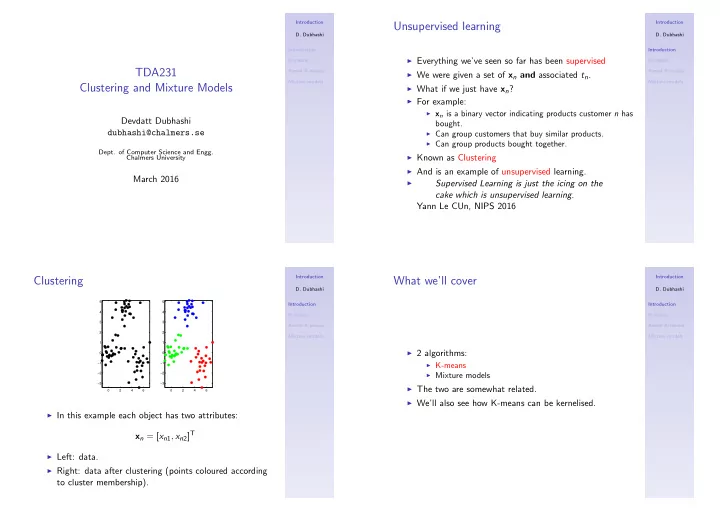
Clustering

2 4 6 −3 −2 −1 1 2 3 4 5 2 4 6 −3 −2 −1 1 2 3 4 5

◮ In this example each object has two attributes:

xn = [xn1, xn2]T

◮ Left: data. ◮ Right: data after clustering (points coloured according

to cluster membership).

Introduction

• D. Dubhashi

Introduction K-means Kernel K-means Mixture models

What we’ll cover

◮ 2 algorithms:

◮ K-means ◮ Mixture models

◮ The two are somewhat related. ◮ We’ll also see how K-means can be kernelised.

SLIDE 2

Introduction

• D. Dubhashi

Introduction K-means Kernel K-means Mixture models

K-means

◮ Assume that there are K clusters. ◮ Each cluster is defined by a position in the input space:

µk = [µk1, µk2]T

◮ Each xn is assigned to its closest cluster:

−2 2 4 6 −6 −4 −2 2 4 6

x1 x2 ◮ Distance is normally Euclidean distance:

dnk = (xn − µk)T(xn − µk)

Introduction

• D. Dubhashi

Introduction K-means Kernel K-means Mixture models

How do we find µk?

◮ No analytical solution – we can’t write down µk as a

function of X.

◮ Use an iterative algorithm:

• 1. Guess µ1, µ2, . . . , µK
• 2. Assign each xn to its closest µk
• 3. znk = 1 if xn assigned to µk (0 otherwise)
• 4. Update µk to average of xns assigned to µk:

µk = N

n=1 znkxn

N

n=1 znk

• 5. Return to 2 until assignments do not change.

◮ Algorithm will converge....it will reach a point where the

assignments don’t change.

Introduction

• D. Dubhashi

Introduction K-means Kernel K-means Mixture models

K-means – example

−2 2 4 6 −6 −4 −2 2 4 6

x1 x2

◮ Cluster means randomly assigned (top left). ◮ Points assigned to their closest mean.

Introduction

• D. Dubhashi

Introduction K-means Kernel K-means Mixture models

K-means – example

−2 2 4 6 −6 −4 −2 2 4 6

x1 x2

◮ Cluster means updated to mean of assigned points.

SLIDE 3

Introduction

• D. Dubhashi

Introduction K-means Kernel K-means Mixture models

K-means – example

−2 2 4 6 −6 −4 −2 2 4 6

x1 x2

◮ Points re-assigned to closest mean.

Introduction

• D. Dubhashi

Introduction K-means Kernel K-means Mixture models

K-means – example

−2 2 4 6 −6 −4 −2 2 4 6

x1 x2

◮ Cluster means updated to mean of assigned points.

Introduction

• D. Dubhashi

Introduction K-means Kernel K-means Mixture models

K-means – example

−2 2 4 6 −6 −4 −2 2 4 6

x1 x2

◮ Solution at convergence.

Introduction

• D. Dubhashi

Introduction K-means Kernel K-means Mixture models

Two Issues with K-Means

◮ What value of k should we use? ◮ How should we pick the initial centers? ◮ Both these significantly affect resulting clustering.

SLIDE 4

Introduction

• D. Dubhashi

Introduction K-means Kernel K-means Mixture models

Initializing Centers

◮ Pick k random points. ◮ Pick k points at random from input points. ◮ Assign points at random to k groups and then take

centers of these groups.

◮ Pick a random input point for first center, next center

at a point as far away from this as possible, next as far away from first two ...

Introduction

• D. Dubhashi

Introduction K-means Kernel K-means Mixture models

k–Means++ (D. Arthur and S. Vassilvitskii (2007)

◮ Start with C1 := {x} where x is chosen at random from

input points.

◮ For i ≥ 2, pick a point x according to a probability

distribution νi: νi(x) = d2(x, Ci−1)

• y d2(y, Ci−1)

and set Ci := Ci−1 ∪ {x}. Gives a provably good O(log n) approximation to optimal clustering.

Introduction

• D. Dubhashi

Introduction K-means Kernel K-means Mixture models

Choosing k

◮ Intra-cluster variance:

Wk := 1 |Ck|

• x∈Ck

(x − µk)2.

◮ W := k Wk. ◮ Pick k to minimize Wk ◮ Elbow heuristic, Gap Statistic ...

Introduction

• D. Dubhashi

Introduction K-means Kernel K-means Mixture models

Sum of Norms (SON) Convex Relaxation

SON Relaxation (Lindsten et al 2011)

min

µ xi − µi2 + λ

• i<j

µi − µj2.

◮ If you take only first term ... ◮ ... µi = xi for all i. ◮ If you take only second term ... ◮ ... µi = µj for all i, j. ◮ By varying λ, we steer between these two extremes. ◮ Do not need to know k in advance and do not need to

do careful intialization.

◮ Fast scalable algorithm with guarantees under

submission later today to ICML ...

SLIDE 5

Introduction

• D. Dubhashi

Introduction K-means Kernel K-means Mixture models

When does K-means break?

−1.5 −1 −0.5 0.5 1 1.5 −1.5 −1 −0.5 0.5 1 1.5

x1 x2

◮ Data has clear cluster structure. ◮ Outer cluster can not be represented as a single point.

Introduction

• D. Dubhashi

Introduction K-means Kernel K-means Mixture models

When does K-means break?

−1.5 −1 −0.5 0.5 1 1.5 −1.5 −1 −0.5 0.5 1 1.5

x1 x2

◮ Data has clear cluster structure. ◮ Outer cluster can not be represented as a single point.

Introduction

• D. Dubhashi

Introduction K-means Kernel K-means Mixture models

Kernelising K-means

◮ Maybe we can kernelise K-means? ◮ Distances:

(xn − µk)T(xn − µk)

◮ Cluster means:

µk = N

m=1 zmkxm

N

m=1 zmk ◮ Distances can be written as (defining Nk = n znk):

(xn−µk)T(xn−µk) =

• xn − N−1

k N

• m=1

zmkxm T xn − N−1

k N

• m=1

zmkxm

• Introduction
• D. Dubhashi

Introduction K-means Kernel K-means Mixture models

Kernelising K-means

◮ Multiply out:

xT

n xn − 2N−1 k N

• m=1

zmkxT

mxn + N−2 k

• m,l

zmkzlkxT

mxl ◮ Kernel substitution:

k(xn, xn)−2N−1

k N

• m=1

zmkk(xn, xm)+N−2

k N

• m,l=1

zmkzlkk(xm, xl)

SLIDE 6

Introduction

• D. Dubhashi

Introduction K-means Kernel K-means Mixture models

Kernel K-means

◮ Algorithm:

• 1. Choose a kernel and any necessary parameters.
• 2. Start with random assignments znk.
• 3. For each xn assign it to the nearest ‘center’ where

distance is defined as: k(xn, xn)−2N−1

k N

• m=1

zmkk(xn, xm)+N−2

k N

• m,l=1

zmkzlkk(xm, xl)

• 4. If assignments have changed, return to 3.

◮ Note – no µk. This would be N−1 k

• n znkφ(xn) but we

don’t know φ(xn) for kernels. We only know φ(xn)Tφ(xm) (last week)...

Introduction

• D. Dubhashi

Introduction K-means Kernel K-means Mixture models

Kernel K-means – example

−1.5 −1 −0.5 0.5 1 1.5 −1.5 −1 −0.5 0.5 1 1.5

x1 x2

◮ Continue re-assigning until convergence.

Introduction

• D. Dubhashi

Introduction K-means Kernel K-means Mixture models

Kernel K-means – example

−1.5 −1 −0.5 0.5 1 1.5 −1.5 −1 −0.5 0.5 1 1.5

x1 x2

◮ Continue re-assigning until convergence.

Introduction

• D. Dubhashi

Introduction K-means Kernel K-means Mixture models

Kernel K-means – example

−1.5 −1 −0.5 0.5 1 1.5 −1.5 −1 −0.5 0.5 1 1.5

x1 x2

◮ Continue re-assigning until convergence.

SLIDE 7

Introduction

• D. Dubhashi

Introduction K-means Kernel K-means Mixture models

Kernel K-means

◮ Makes simple K-means algorithm more flexible. ◮ But, have to now set additional parameters. ◮ Very sensitive to initial conditions – lots of local optima.

Introduction

• D. Dubhashi

Introduction K-means Kernel K-means Mixture models

K-means – summary

◮ Simple (and effective) clustering strategy. ◮ Converges to (local) minima of:

• n
• k

znk(xn − µk)T(xn − µk)

◮ Sensitive to initialisation. ◮ How do we choose K?

◮ Tricky: Quantity above always decreases as K increases. ◮ Can use CV if we have a measure of ‘goodness’. ◮ For clustering these will be application specific. Introduction

• D. Dubhashi

Introduction K-means Kernel K-means Mixture models

Mixture models – thinking generatively

−2 −1 1 2 3 4 5 −6 −4 −2 2 4 6

x1 x2

◮ Could we hypothesis a model that could have created

this data?

◮ Each xn seems to have come from one of three

distributions.

Introduction

• D. Dubhashi

Introduction K-means Kernel K-means Mixture models

A generative model

◮ Assumption:Each xn comes from one of different K

distributions.

◮ To generate X: ◮ For each n:

• 1. Pick one of the K components.
• 2. Sample xn from this distribution.

◮ We already have X ◮ Define parameters of all these distributions as ∆. ◮ We’d like to reverse-engineer this process learn ∆ which

we can then use to find which component each point came from.

◮ Maximise the likelihood!

SLIDE 8

Introduction

• D. Dubhashi

Introduction K-means Kernel K-means Mixture models

Mixture model likelihood

◮ Let the kth distribution have pdf:

p(xn|znk = 1, ∆k)

◮ We want the likelihood:

p(X|∆)

◮ First, factorise:

p(X|∆) =

N

• i=1

p(xn|∆)

◮ Then, un-marginalise k:

p(X|∆) =

N

• i=1

K

• k=1

p(xn, znk = 1|∆) =

N

• i=1

K

• k=1

p(xn|znk = 1, ∆k)p(znk = 1|∆)

Introduction

• D. Dubhashi

Introduction K-means Kernel K-means Mixture models

Mixture model likelihood

◮ So, we have a likelihood:

p(X|∆) =

N

• i=1

K

• k=1

p(xn|znk = 1, ∆k)p(znk = 1|∆)

◮ And we want to find ∆. ◮ So:

argmax

∆ N

• i=1

K

• k=1

p(xn|znk = 1, ∆k)p(znk = 1|∆)

◮ Logging made this easier before, so let’s try it:

argmax

∆ N

• n=1

log

K

• k=1

p(xn|znk = 1, ∆k)p(znk = 1|∆)

◮ Log of a sum is bad – we need some help....

Introduction

• D. Dubhashi

Introduction K-means Kernel K-means Mixture models

Jensen’s inequality

log Ep(x) {f (x)} ≥ Ep(x) {log f (x)}

◮ How does this help us? ◮ Our log likelihood:

L =

N

• n=1

log

K

• k=1

p(xn|znk = 1, ∆k)p(znk = 1|∆)

◮ Add a (arbitrary looking) distribution q(znk = 1) (s.t.

• k q(znk = 1) = 1):

L =

N

• n=1

log

K

• k=1

q(znk = 1) q(znk = 1)p(xn|znk = 1, ∆k)p(znk = 1|∆)

Introduction

• D. Dubhashi

Introduction K-means Kernel K-means Mixture models

Jensen’s inequality

L =

N

• n=1

log

K

• k=1

q(znk = 1) q(znk = 1)p(xn|znk = 1, ∆k)p(znk = 1|∆)

◮ We now have an expectation:

L =

N

• n=1

log Eq(znk=1)

• 1

q(znk = 1)p(xn|znk = 1, ∆k)p(znk = 1|∆)

• ◮ So, using Jensen’s:

L ≥

N

• n=1

Eq(znk=1)

• log

1 q(znk = 1)p(xn|znk = 1, ∆k)p(znk = 1|∆)

• =

N

• n=1

K

• k=1

q(znk = 1) log

• 1

q(znk = 1)p(xn|znk = 1, ∆k)p(znk = 1|∆)

SLIDE 9

Introduction

• D. Dubhashi

Introduction K-means Kernel K-means Mixture models

Lower bound on log-likelihood

L ≥

N

• n=1

K

• k=1

q(znk = 1) log

• 1

q(znk = 1)p(xn|znk = 1, ∆k)p(znk = 1|∆)

• =

N

• n=1

K

• k=1

q(znk = 1) log p(znk = 1|∆) + . . .

N

• n=1

K

• k=1

q(znk = 1) log p(xn|znk = 1, ∆k) − . . .

N

• n=1

K

• k=1

q(znk = 1) log q(znk = 1)

◮ Define qnk = q(znk = 1), πk = p(znk = 1|∆) (both just

scalars).

◮ Differentiate lower bound w.r.t qnk, πk and ∆k and set to

zero to obtain iterative update equations.

Introduction

• D. Dubhashi

Introduction K-means Kernel K-means Mixture models

Optimising lower bound

◮ Updates for ∆k, πk will depend on qnk. ◮ Update qnk and then use these values to update ∆k

and πk etc.

◮ This is a form of the Expectation-Maximisation

algorithm (EM) but we’ve derived it differently.

◮ Best illustrated with an example....

Introduction

• D. Dubhashi

Introduction K-means Kernel K-means Mixture models

Gaussian mixture model

◮ Assume component distributions are Gaussians with

diagonal covariance: p(xn|znk = 1, µk, σ2

k) = N(µ, σ2I) ◮ Update for πk. Relevant bit of bound:

• n,k

qnkπk

◮ Now, we have a constraint: k πk = 1. So, add a

Lagrangian:

• n,k

qnk log πk − λ

• k

πk − 1

• ◮ Differentiate and set to zero:

∂ ∂πk = 1 πk

• n

qnk − λ = 0

Introduction

• D. Dubhashi

Introduction K-means Kernel K-means Mixture models

◮ Re-arrange:

• n

qnk = λπk

◮ Sum both sides over k to find λ:

• n,k

qnk = λ × 1

◮ Substitute and re-arrange:

πk =

• n qnk
• n,j qnj

= 1 N

• k

qnk

SLIDE 10

Introduction

• D. Dubhashi

Introduction K-means Kernel K-means Mixture models

Update for qnk

◮ Now for qnk. Whole bound is relevant. ◮ Add Lagrange term −λ( k qnk − 1) ◮ Differentiate:

∂ ∂qnk = log πk +log p(xn|znk = 1, ∆k)−(log qnk +1)−λ

◮ Re-arranging (λ′ = f (λ)):

πkp(xn|znk = 1, ∆k) = λ′qnk

◮ Sum over k to find λ′ and re-arrange:

qnk = πkp(xn|znk = 1, ∆k) K

j=1 πjp(xn|znj = 1, ∆j)

Introduction

• D. Dubhashi

Introduction K-means Kernel K-means Mixture models

Updates for µk and σ2

k

◮ These are easier – no constraints. ◮ Differentiate the following and set to zero (D is

dimension of xn):

• n,k

qnk log

• 1

(2πσ2

k)D/2 exp

• − 1

2σ2

k

(xn − µk)T(xn − µk)

• ◮ Result:

µk =

• n qnkxn
• n qnk

σ2

k

=

• n qnk(xn − µk)T(xn − µk)

D

n qnk

Introduction

• D. Dubhashi

Introduction K-means Kernel K-means Mixture models

Mixture model optimisation – algorithm

◮ Following optimisation algorithm:

• 1. Guess µk, σ2

k, πk

• 2. Compute qnk
• 3. Update µk, σ2

k

• 4. Update πk
• 5. Return to 2 unless parameters are unchanged.

◮ Guaranteed to converge to a local maximum of the

lower bound.

◮ Note the similarity with kmeans.

Introduction

• D. Dubhashi

Introduction K-means Kernel K-means Mixture models

Algorithm in operation

x1 x2

−2 2 4 −6 −4 −2 2 4 6 ◮ Initial parameter values.

SLIDE 11

Introduction

• D. Dubhashi

Introduction K-means Kernel K-means Mixture models

x1 x2

−2 2 4 −6 −4 −2 2 4 6 ◮ Update qnk and then other parameters.

Introduction

• D. Dubhashi

Introduction K-means Kernel K-means Mixture models

x1 x2

−2 2 4 −6 −4 −2 2 4 6 ◮ Update qnk and then other parameters.

Introduction

• D. Dubhashi

Introduction K-means Kernel K-means Mixture models

x1 x2

−2 2 4 −6 −4 −2 2 4 6 ◮ Solution at convergence.

Introduction

• D. Dubhashi

Introduction K-means Kernel K-means Mixture models

Mixture model clustering

◮ So, we’ve got the parameters, but what about the

assignments?

◮ Which points came from which distributions? ◮ qnk is the probability that xn came from distribution k.

qnk = P(znk = 1|xn, X, t)

◮ Can stick with probabilities or assign each xn to it’s

most likely component.

SLIDE 12

Introduction

• D. Dubhashi

Introduction K-means Kernel K-means Mixture models

Mixture model clustering

−2 2 4 −6 −4 −2 2 4 6

x1 x2

◮ Points assigned to the cluster with the highest qnk

value.

Introduction

• D. Dubhashi

Introduction K-means Kernel K-means Mixture models

Mixture model – issues

◮ How do we choose K? ◮ What happens when we increase it? ◮ K = 10

x1 x2

−2 2 4 −6 −4 −2 2 4 6

Introduction

• D. Dubhashi

Introduction K-means Kernel K-means Mixture models

Likelihood increase

2 4 6 8 10 −400 −390 −380 −370 −360 −350 −340 −330

K Log likelihood

◮ Likelihood always increases as σ2 k decreases.

Introduction

• D. Dubhashi

Introduction K-means Kernel K-means Mixture models

What can we do?

◮ What can we do? ◮ Cross-validation...

2 4 6 8 10 −46 −45 −44 −43 −42 −41 −40 −39 −38

K Held out Log likelihood

◮ 10-fold CV. Maximum is close to true value (3) ◮ 5 might be better for this data....

SLIDE 13

Introduction

• D. Dubhashi

Introduction K-means Kernel K-means Mixture models

Mixture models – other distributions

◮ We’ve seen Gaussian distributions. ◮ Can actually use anything.... ◮ As long as we can define p(xn|znk = 1, ∆k) ◮ e.g. Binary data:

Introduction

• D. Dubhashi

Introduction K-means Kernel K-means Mixture models

Binary example

◮ xn = [0, 1, 0, 1, 1, . . . , 0, 1]T (D dimensions) ◮ p(xn|znk = 1, ∆k) = D d=1 pxnd kd (1 − pkd)1−xnd ◮ Updates for pkd are:

pkd =

• n qnkxnd
• n qnk

◮ qnk and πk are the same as before... ◮ Initialise with random pkd (0 ≤ pkd ≤ 1)

Introduction

• D. Dubhashi

Introduction K-means Kernel K-means Mixture models

Results

◮ K = 5 clusters. ◮ Clear structure present.

Introduction

• D. Dubhashi

Introduction K-means Kernel K-means Mixture models

Summary

◮ Introduced two clustering methods. ◮ K-means

◮ Very simple. ◮ Iterative scheme. ◮ Can be kernelised. ◮ Need to choose K.

◮ Mixture models

◮ Create a model of each class (similar to Bayes classifier) ◮ Iterative sceme (EM) ◮ Can use any distribution for the components. ◮ Can set K by cross-validation (held-out likelihood) ◮ State-of-the-art: Don’t need to set K – treat as a

variable in a Bayesian sampling scheme.