Univariate Smoothing Overview Problem Definition & Interpolation - PowerPoint PPT Presentation

Univariate Smoothing Overview Problem Definition & Interpolation • Problem definition • Smoothing Problem: Given a data set with a single input variable x , find the best function ˆ g ( x ) that minimizes the • Interpolation prediction error on new inputs (probably not in the data set) • Polynomial smoothing • Interpolation Problem: Same as the smoothing problem except • Cubic splines the model is subject to the constraint ˆ g ( x i ) = y i for every • Basis splines input-output pair ( x i , y i ) in the data set • Smoothing splines – Linear Interpolation : Use a line between each pair of points • Bayes’ rule – Nearest Neighbor Interpolation : Find the nearest input in the data set and use the corresponding output as an • Density estimation approximate fit • Kernel smoothing – Polynomial Interpolation : Fit a polynomial of order n − 1 to • Local averaging g ( x ) = � n i =1 w i x i − 1 input output data: ˆ • Weighted least squares – Cubic Spline Interpolation : Fit a cubic polynomial with • Local linear models continuous second derivatives in between each pair of points (more on this later) • Prediction error estimates J. McNames Portland State University ECE 4/557 Univariate Smoothing Ver. 1.25 1 J. McNames Portland State University ECE 4/557 Univariate Smoothing Ver. 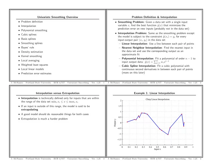1.25 2 Interpolation versus Extrapolation Example 1: Linear Interpolation • Interpolation is technically defined only for inputs that are within Chirp Linear Interpolation 2 the range of the data set min i x i ≤ x ≤ max i x i • If an input is outside of this range, the model is said to be 1.5 extrapolating 1 • A good model should do reasonable things for both cases 0.5 • Extrapolation is much a harder problem Output y 0 −0.5 −1 −1.5 −2 0 0.1 0.2 0.3 0.4 0.5 0.6 0.7 0.8 0.9 1 Input x J. McNames Portland State University ECE 4/557 Univariate Smoothing Ver. 1.25 3 J. McNames Portland State University ECE 4/557 Univariate Smoothing Ver. 1.25 4

Example 1: MATLAB Code % ================================================ % Nearest Neighbor Interpolation % ================================================ figure; %function [] = Interpolation (); FigureSet (1,’LTX ’); yh = interp1(x,y,xt ,’nearest ’); close all; h = plot(xt ,yh ,’b’,x,y,’r.’); set(h,’MarkerSize ’ ,8); N = 15; set(h,’LineWidth ’,1.2); rand(’state ’ ,2); xlabel(’Input x’); x = rand(N ,1); ylabel(’Output y’); y = sin (2* pi *2* x. ^2) + 0.2*randn(N ,1); title(’Chirp Nearest Neighbor Interpolation ’); xt = (0:0 .0001 :1) ’; % Test inputs set(gca ,’Box ’,’Off ’); grid on; % ================================================ axis ([0 1 -2 2]); % Linear Interpolation AxisSet (8); % ================================================ print -depsc InterpolationNearestNeighbor; figure; FigureSet (1,’LTX ’); % ================================================ yh = interp1(x,y,xt ,’linear ’); % Polynomial Interpolation h = plot(xt ,yh ,’b’,x,y,’r.’); % ================================================ set(h,’MarkerSize ’ ,8); A = zeros(N,N); set(h,’LineWidth ’,1.2); for cnt = 1: size(A,2), xlabel(’Input x’); A(:,cnt) = x.^(cnt -1); ylabel(’Output y’); end; title(’Chirp Linear Interpolation ’); w = pinv(A)*y; set(gca ,’Box ’,’Off ’); At = zeros(length(xt),N); grid on; for cnt = 1: size(A,2), axis ([0 1 -2 2]); At(:,cnt) = xt. ^(cnt -1); AxisSet (8); end; print -depsc InterpolationLinear; J. McNames Portland State University ECE 4/557 Univariate Smoothing Ver. 1.25 5 J. McNames Portland State University ECE 4/557 Univariate Smoothing Ver. 1.25 6 yh = At*w; grid on; axis ([0 1 -2 2]); figure; AxisSet (8); FigureSet (1,’LTX ’); print -depsc InterpolationCubicSpline ; h = plot(xt ,yh ,’b’,x,y,’r.’); set(h,’MarkerSize ’ ,8); % ================================================ set(h,’LineWidth ’,1.2); % Cubic Spline Interpolation xlabel(’Input x’); % ================================================ ylabel(’Output y’); figure; title(’Chirp Polynomial Interpolation ’); FigureSet (1,’LTX ’); set(gca ,’Box ’,’Off ’); yt = sin (2* pi *2* xt. ^2); grid on; h = plot(xt ,yt ,’b’,x,y,’r.’); axis ([0 1 -2 2]); set(h,’MarkerSize ’ ,8); set(h,’LineWidth ’,1.2); AxisSet (8); xlabel(’Input x’); ylabel(’Output y’); print -depsc InterpolationPolynomial; title(’Chirp Optimal Model ’); set(gca ,’Box ’,’Off ’); % ================================================ grid on; % Cubic Spline Interpolation axis ([0 1 -2 2]); % ================================================ AxisSet (8); figure; print -depsc InterpolationOptimalModel ; FigureSet (1,’LTX ’); yh = spline(x,y,xt); h = plot(xt ,yh ,’b’,x,y,’r.’); set(h,’MarkerSize ’ ,8); set(h,’LineWidth ’,1.2); xlabel(’Input x’); ylabel(’Output y’); title(’Chirp Cubic Spline Interpolation ’); set(gca ,’Box ’,’Off ’); J. McNames Portland State University ECE 4/557 Univariate Smoothing Ver. 1.25 7 J. McNames Portland State University ECE 4/557 Univariate Smoothing Ver. 1.25 8

Example 2: Nearest Neighbor Interpolation Example 2: MATLAB Code Same data set and test inputs as linear interpolation example. Chirp Nearest Neighbor Interpolation 2 1.5 1 0.5 Output y 0 −0.5 −1 −1.5 −2 0 0.1 0.2 0.3 0.4 0.5 0.6 0.7 0.8 0.9 1 Input x J. McNames Portland State University ECE 4/557 Univariate Smoothing Ver. 1.25 9 J. McNames Portland State University ECE 4/557 Univariate Smoothing Ver. 1.25 10 Example 3: Polynomial Interpolation Example 3: MATLAB Code Same data set and test inputs as linear interpolation example. Chirp Polynomial Interpolation 2 1.5 1 0.5 Output y 0 −0.5 −1 −1.5 −2 0 0.1 0.2 0.3 0.4 0.5 0.6 0.7 0.8 0.9 1 Input x J. McNames Portland State University ECE 4/557 Univariate Smoothing Ver. 1.25 11 J. McNames Portland State University ECE 4/557 Univariate Smoothing Ver. 1.25 12

Example 4: Cubic Spline Interpolation Example 4: MATLAB Code Same data set and test inputs as linear interpolation example. Chirp Cubic Spline Interpolation 2 1.5 1 0.5 Output y 0 −0.5 −1 −1.5 −2 0 0.1 0.2 0.3 0.4 0.5 0.6 0.7 0.8 0.9 1 Input x J. McNames Portland State University ECE 4/557 Univariate Smoothing Ver. 1.25 13 J. McNames Portland State University ECE 4/557 Univariate Smoothing Ver. 1.25 14 Interpolation Comments Smoothing • There are an infinite number of functions that satisfy the • For the smoothing problem, even the constraint is relaxed interpolation constraint: ˆ g ( x i ) ≈ y i ∀ i ˆ g ( x i ) = y i ∀ i • The data set can be merely suggesting what the model output • Of course, we would like to choose the model that minimizes the should be approximately at some specified points prediction error • We need another constraint or assumption about the relationship • Given only data, there is no way to do this exactly between x and y to have enough constraints to uniquely specify the model • Our data set only specifies what ˆ g ( x ) should be at specific points • What should it be in between these points? • In practice, the method of interpolation is usually chosen by the user J. McNames Portland State University ECE 4/557 Univariate Smoothing Ver. 1.25 15 J. McNames Portland State University ECE 4/557 Univariate Smoothing Ver. 1.25 16

Smoothing Assumptions and Statistical Model Example 5: Interpolation Optimal Model y = g ( x ) + ε Chirp Optimal Model 2 • Generally we assume that the data was generated from the statistical model above 1.5 • ε i is a random variable with the following assumed properties 1 – Zero mean: E[ ε ] = 0 0.5 – ε i and ε j are independently distributed for i � = j Output y – ε i is identically distributed 0 • The two additional assumptions are usually made for the −0.5 smoothing problem −1 – g ( x ) is continuous – g ( x ) is smooth −1.5 −2 0 0.1 0.2 0.3 0.4 0.5 0.6 0.7 0.8 0.9 1 Input x J. McNames Portland State University ECE 4/557 Univariate Smoothing Ver. 1.25 17 J. McNames Portland State University ECE 4/557 Univariate Smoothing Ver. 1.25 18 Smoothing Bias-Variance Tradeoff Recall that y i = g ( x i ) + ε i � g ( x )) 2 � MSE( x ) = E ( g ( x ) − ˆ � g ( x )]) 2 � g ( x )]) 2 + E • When we add noise, we can drop the interpolation constraint: = ( g ( x ) − E[ˆ (ˆ g ( x ) − E[ˆ ˆ g ( x i ) = y i ∀ i Bias 2 + Variance = • But we still want ˆ g ( · ) to be consistent with (i.e. close to) the data: ˆ g ( x i ) ≈ y i • Fundamental smoother tradeoff: – Smoothness of the estimate ˆ g ( x ) • The methods we will discuss are biased in favor of models that are smooth – Fit to the data • This can also be framed as a bias-variance tradeoff J. McNames Portland State University ECE 4/557 Univariate Smoothing Ver. 1.25 19 J. McNames Portland State University ECE 4/557 Univariate Smoothing Ver. 1.25 20