Univariate point-level modeling Basic Model: Y ( s ) = x T ( s ) + - - PowerPoint PPT Presentation

Univariate point-level modeling

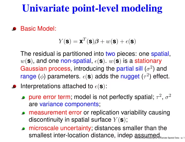
Basic Model:

Y (s) = xT (s)β + w(s) + ǫ(s)

The residual is partitioned into two pieces: one spatial,

w(s), and one non-spatial, ǫ(s). w(s) is a stationary

Gaussian process, introducing the partial sill (σ2) and range (φ) parameters. ǫ(s) adds the nugget (τ2) effect. Interpretations attached to ǫ(s): pure error term; model is not perfectly spatial; τ2, σ2 are variance components; measurement error or replication variability causing discontinuity in spatial surface Y (s); microscale uncertainty; distances smaller than the smallest inter-location distance, indep assumed.

Hierarchical Modeling for Univariate Spatial Data – p. 1

Isotropic models

Suppose we have data Y (si), i = 1, . . . , n, and let Y = (Y (s1), . . . , Y (sn))T. Gaussian kriging models are special cases of of the general linear model, with a particular specification of the dispersion matrix

Σ = σ2H(φ) + τ2I. Hij = ρ(si − sj; φ), where ρ is a valid (and typically

isotropic) correlation function. Setting θ = (β, σ2, τ2, φ)T (not a high dim problem), we require a prior p(θ), so the posterior is:

p(θ|y) ∝ f(y|θ)p(θ)

Hierarchical Modeling for Univariate Spatial Data – p. 2

Likelihood and priors

The likelihood is given by: Y|θ ∼ N(Xβ, σ2H(φ) + τ2I) Typically, independent priors are chosen for the parameters:

p(θ) = p(β)p(σ2)p(τ2)p(φ)

Useful candidates are multivariate normal for β, and inverse gamma for σ2 and τ2. Specification of p(φ) depends upon choice of ρ function; a uniform or discrete prior is usually selected.

Hierarchical Modeling for Univariate Spatial Data – p. 3

Priors cont.

Informativeness: p(β) can be “flat" (improper) Without nugget, τ2, can’t identify both σ2 and φ (Zhang, 2004). With Matérn, can identify the product. So an informative prior on at least one of these parameters With τ2, then φ and at least one of σ2 and τ2 require informative priors. Suppose a Matérn covariance function. If the prior on

β, σ2, φ is of the form π(φ)

(σ2)α with π(·) uniform, then,

improper posterior if α < 2 Shows the problem with using IG(ǫ, ǫ) priors for σ2 - “nearly” improper. Safer is IG(a, b) with a ≥ 1

Hierarchical Modeling for Univariate Spatial Data – p. 4

Hierarchical modeling

Foregoing is really a hierarchical setup by considering a conditional likelihood on the spatial random effects w = (w(s1), . . . , w(sn)). First stage: Y|θ, w ∼ N(Xβ + w, τ2I) The Y (si) are conditionally independent given the

w(si)’s.

Second stage: w|σ2, φ ∼ N(0, σ2H(φ)) Third stage: priors on (β, τ2, σ2, φ)

Hierarchical Modeling for Univariate Spatial Data – p. 5

Computing the posterior

We seek the marginal posterior p(θ|y), which is the same under the original and hierarchical settings Choice: Fit as f(y|θ)p(θ) or as f(y|θ, w)p(w|θ)p(θ). Fitting the marginal model is computationally more stable: lower dimensional sampler (no w’s);

σ2H(φ) + τ2I more stable than σ2H(φ)

BUT the conditional model allows conjugate full conditionals for σ2, τ2 (inverse gamma), β, and w (Gaussian) – easy updates! Marginalized model will need Metropolis updates for σ2,

τ2, and φ. But these usually work well and often

converge faster than the full Gibbs updates.

Hierarchical Modeling for Univariate Spatial Data – p. 6

Where are the w’s?

Interest often lies in the spatial surface w|y (pattern of spatial adjustment) Have we lost the w’s with the marginalized sampling? No: They are easily recovered via composition sampling:

p(w|y) =

• p(w|θ, y)p(θ|y)dθ

Note that

p(w|θ, y) ∝ f(y|w, β, τ2)p(w|σ2, φ)

is a multivariate normal distribution, resulting in easy composition sampling, in fact 1-1 with posterior samples of θ

Hierarchical Modeling for Univariate Spatial Data – p. 7

Spatial prediction (Bayesian kriging)

Prediction of Y (s0) at a new site s0 with associated covariates x0 ≡ x(s0). Predictive distribution:

p(y(s0)|y, X, x0) =

• p(y(s0), θ|y, X, x0)dθ

=

• p(y(s0)|y, θ, X, x0)p(θ|y, X)dθ

p(y(s0)|y, θ, X, x0) is normal since p(y0, y|θ, X, x0) is! ⇒ easy Monte Carlo estimate using composition with

Gibbs draws θ(1), . . . , θ(G): For each θ(g) drawn from

p(θ|y, X), draw Y (s0)(g) from p(y(s0)|y, θ(g), X, x0).

Hierarchical Modeling for Univariate Spatial Data – p. 8

Joint prediction

Suppose we want to predict at a set of m sites, say

S0 = {s01, . . . , s0m}.

We could individually predict each site “independently” using method of the previous slide BUT joint prediction may be of interest, e.g., bivariate predictive distributions to reveal pairwise dependence, to reflect posterior associations in the realized surface: Form the unobserved vector Y0 = (Y(s01), . . . , Y(s0m)), with X0 as covariate matrix for S0, and compute

p(y0|y, X, X0) =

• p(y0|y, θ, X, X0)p(θ|y, X)

Again, posterior sampling using composition sampling.

Hierarchical Modeling for Univariate Spatial Data – p. 9

Spatial Generalized Linear Models

Some data sets preclude Gaussian modeling; Y (s) need not be continuous Example: Y (s) is a binary or count variable Presence/absence of a species at a location; abundance of a species at a location precipitation or deposition was measurable or not number of insurance claims by residents of a single family home at s Land use classification at a location (not ordinal)

⇒ replace Gaussian likelihood by an appropriate

exponential family member if possible See Diggle Tawn and Moyeed (1998)

Hierarchical Modeling for Univariate Spatial Data – p. 10

Spatial GLM (cont’d)

First stage: Y (si) are conditionally independent given β and w(si) with f(y(si)|β, w(si), γ) an appropriate non-Gaussian likelihood such that

g(E(Y (si))) = η(si) = xT (si)β + w(si) ,

where η is a canonical link function (such as a logit) and

γ is a dispersion parameter.

Second stage: Model w(s) as a Gaussian process: w ∼ N(0, σ2H(φ)) Third stage: Priors and hyperpriors. Lose conjugacy between first and second stage; not sensible to add a pure error term

Hierarchical Modeling for Univariate Spatial Data – p. 11

Spatial GLM: comments

Spatial random effects in the transformed mean with continuous covariates encourages the means of spatial variables at proximate locations to be close to each

• ther

Marginal spatial dependence is induced between, say,

Y (s) and Y (s′), but the observed Y (s) and Y (s′) need

not be close. No smoothness in Y (s) surface Our second stage modeling is attractive for spatial explanation in the mean First stage modeling is better for encouraging proximate

• bservations to be close.

Note that this approach offers a valid joint distribution for the Y (si), but not a spatial process model; we need not achieve a consistent stochastic process for the uncountable collection of Y (s) values

Hierarchical Modeling for Univariate Spatial Data – p. 12