Unit 6: Introduction to linear regression 1. Introduction to - - PowerPoint PPT Presentation

Unit 6: Introduction to linear regression

• 1. Introduction to regression

STA 104 - Summer 2017

Duke University, Department of Statistical Science

• Prof. van den Boom

Slides posted at http://www2.stat.duke.edu/courses/Summer17/sta104.001-1/

Announcements ▶ MT 2 grades have been posted today!

The CDC monitors the physical activity level of Americans. A recent survey on a random sample of 23,129 Americans yielded a 95% confidence interval of 61.1% to 62.9% for the proportion of Americans who walk for at least 10 minutes per

• day. Which is the most accurate statement?
• A. 95% of random samples of 23,129 Americans will yield confidence

intervals between 61.1% and 62.9%.

• B. This interval does not support the claim that less than 50% of Americans

walk at least 10 minutes per day.

• C. We are 95% confident that each American walks for at least 10 minutes

per day on 61.1% to 62.9% of the days.

• D. Between 61.1% and 62.9% of random samples of 23,129 Americans are

expected to yield confidence intervals that contain the true proportion of Americans who walk for at least 10 minutes per day.

• E. 95% of the time the true proportion of Americans who walk for at least 10

minutes per day is between 61.1% to 62.9%. For post-hoc tests of the results of an ANOVA we use a corrected alpha or significance level. If we want an overall type 1 error rate of 5%, what should the alpha be for the individual pairwise tests if the number of groups equals 6? Choose the closest option.

• A. 0.16667
• B. 0.00833
• C. 0.00333
• D. 0.05
• E. 0.3

1

Modeling numerical variables ▶ So far we have worked with single numerical and categorical

variables, and explored relationships between numerical and categorical, and two categorical variables.

▶ In this unit we will learn to quantify the relationship between two

numerical variables, as well as modeling numerical response variables using a numerical or categorical explanatory variable.

▶ In the next unit we’ll learn to model numerical variables using

many explanatory variables at once.

2

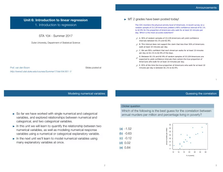
Guessing the correlation

Clicker question

Which of the following is the best guess for the correlation between annual murders per million and percentage living in poverty? (a) -1.52 (b) -0.63 (c) -0.12 (d) 0.02 (e) 0.84

• 14

16 18 20 22 24 26 5 10 15 20 25 30 35 40 % in poverty annual murders per million

3

Guessing the correlation

Clicker question

Which of the following is the best guess for the correlation between annual murders per million and population size? (a) -0.97 (b) -0.61 (c) -0.06 (d) 0.55 (e) 0.97

• 2e+06

4e+06 6e+06 8e+06 5 10 15 20 25 30 35 40 population annual murders per million

4

Assessing the correlation

Clicker question

Which of the following is has the strongest correlation, i.e. correlation coefficient closest to +1 or -1?

• (a)
• (b)
• (c)
• (d)

5

Play the game!

To sharpen your correlation guessing abilities: http://guessthecorrelation.com/

6

Spurious correlations

Remember: correlation does not always imply causation! http://www.tylervigen.com/

7

(2) Least squares line minimizes squared residuals ▶ Residuals are the leftovers from the model fit, and calculated as

the difference between the observed and predicted y: ei = yi − ˆ yi

▶ The least squares line minimizes squared residuals:

– Population data: ˆ y = β0 + β1x – Sample data: ˆ y = b0 + b1x

• 14

16 18 20 22 24 26 5 10 15 20 25 30 35 40 % in poverty annual murders per million

8

(3) Interpreting the last squares line ▶ Slope: For each unit increase in x, y is expected to be

higher/lower on average by the slope. b1 = sy sx R

▶ Intercept: When x = 0, y is expected to equal the intercept.

b0 = ¯ y − b1¯ x

– The calculation of the intercept uses the fact the a regression line always passes through (¯ x,¯ y).

9

Why does the regression line always pass through (¯ x,¯ y)?

▶ If there is no relationship between x and y (b1 = 0), the best

guess for ˆ y for any value of x is ¯ y.

▶ Even when there is a relationship between x and y (b1 ̸= 0), the

best guess for ˆ y when x = ¯ x is still ¯ y.

−1.0 0.0 0.5 1.0 1.5 2.0 −1.5 −0.5 0.5 1.5 x y

• (x, y)

−1.0 0.0 0.5 1.0 1.5 2.0 −2 2 4 x y2

• (x, y)

−1.0 0.0 0.5 1.0 1.5 2.0 −2 2 4 6 8 10 x y3

• (x, y)

10

Application exercise: 6.1 Linear model

See course website for details

11

Clicker question

What is the interpretation of the slope? (a) Each additional percentage in those living in poverty increases number of annual murders per million by 2.56. (b) For each percentage increase in those living in poverty, the number of annual murders per million is expected to be higher by 2.56 on average. (c) For each percentage increase in those living in poverty, the number of annual murders per million is expected to be lower by 29.91 on average. (d) For each percentage increase annual murders per million, the percentage of those living in poverty is expected to be higher by 2.56 on average.

12

Clicker question

Suppose you want to predict annual murder count (per million) for a series of districts that were not included in the dataset. For which of the following districts would you be most comfortable with your prediction? A district where % in poverty = (a) 5% (b) 15% (c) 20% (d) 26% (e) 40%

• 14

16 18 20 22 24 26 5 10 15 20 25 30 35 40 % in poverty annual murders per million

13

A note about the intercept

Sometimes the intercept might be an extrapolation: useful for adjusting the height of the line, but meaningless in the context of the data.

10 20 30 40 50 60 −40 40 80 % in poverty annual murders per million

• 14

Calculating predicted values

By hand: murder = −29.91 + 2.56 poverty The predicted number of murders per million per year for a county with 20% poverty rate is:

• murder = −29.91 + 2.56 × 20 = 21.29

In R:

# load data murder <- read.csv("https://stat.duke.edu/~mc301/data/murder.csv") # fit model m_mur_pov <- lm(annual_murders_per_mil ~ perc_pov, data = murder) # create new data newdata <- data.frame(perc_pov = 20) # predict predict(m_mur_pov, newdata) 1 21.28663 15

Summary of main ideas

• 1. Correlation coefficient describes the strength and direction of

the linear association between two numerical variables

• 2. Least squares line minimizes squared residuals
• 3. Interpreting the least squares line
• 4. Predict, but don’t extrapolate

16