
SLIDE 1
Software Clustering
Decomposing a large software system into meaningful subsystems
Understanding the Structure of Programs is Difficult
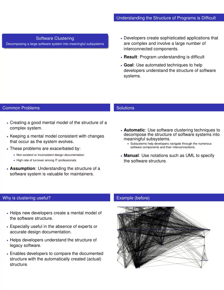
- Developers create sophisticated applications that
are complex and involve a large number of interconnected components.
- Result: Program understanding is difficult
- Goal: Use automated techniques to help
developers understand the structure of software systems. Common Problems
- Creating a good mental model of the structure of a
complex system.
- Keeping a mental model consistent with changes
that occur as the system evolves.
- These problems are exacerbated by:
- Non-existent or inconsistent design documentation
- High rate of turnover among IT professionals
- Assumption: Understanding the structure of a
software system is valuable for maintainers. Solutions
- Automatic: Use software clustering techniques to
decompose the structure of software systems into meaningful subsystems.
- Subsystems help developers navigate through the numerous
software components and their interconnections.
- Manual: Use notations such as UML to specify
the software structure. Why is clustering useful?
- Helps new developers create a mental model of
the software structure.
- Especially useful in the absence of experts or
accurate design documentation.
- Helps developers understand the structure of
legacy software.
- Enables developers to compare the documented